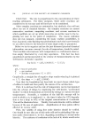
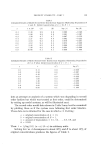
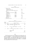
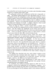
PRODUCT STABILITY--PART I 139 Table I Calculated Results of Model Second Order Kinetic Rate Equation Illustrating Degradation of J and B: Initial Concentration o[ A = 10, B = 1 x t x 102 (A) (B) log (zi) log (B) O. 1 O. 46 0.2 0.98 O.3 1.58 0.4 2.27 O. 5 3.10 0.6 4.12 0.7 5.46 0.8 7.36 O. 9 10.66 99 98 97 96 95 94 93 92 91 0.9 0.996 --0.046 0.8 0.991 --0.097 0.7 0.987 --0.155 0.6 0.982 --0.222 0.5 0.978 --0.301 0.4 0.973 --0.398 0.3 0.968 --0.523 0.2 0.964 --0.699 0.1 0.959 --1.000 Table II Calculated Results of Model Second Order Kinetic Rate Equation Illustrating Degradation of C or D when Initial Concentration of C = D = 1 x t (C) log (C) 0.1 0.11 0.9 0.2 0.25 0.8 0.3 O.43 0.7 0.4 0.67 0.6 0.5 1.00 0.5 0.6 1.50 0.4 0.7 2.33 0.3 0.8 4.00 0.2 0.9 9.00 0.1 -- O. 046 - O. O97 -0. 155 -0 222 --0 301 -0 398 -0 523 -0 699 - 1 000 into an attempt at analysis of a system which was degrading in second order fashion but which was treated as first order, could be determined by setting up model systems, as will be illustrated next. The second order model data shown in Table I may best be examined by plotting them as if the system were following first order kinetics. These data were obtained for the case in which a =• b letting: a = original concentration of A = 10, b -- original concentration of B = 1, x = amount of degradation = 0.1, 0.2, ..., 0.8, 0.9, and k = 2.303. Then: t = •/.• log (0.1) (a-- x) / (b - x) in arbitrary units. Solving for t as A decomposes to about 90% and B to about 10% of original concentrations produces the figures of Table I.

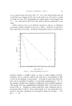
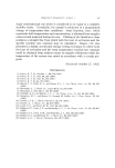
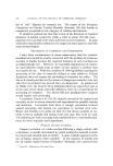
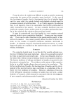
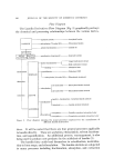
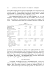
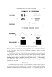
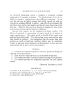
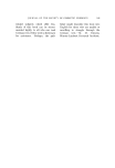
140 JOURNAL OF THE SOCIETY OF COSMETIC CHEMISTS Figure 1 shows the data of Table I graphically. It can be seen that in the case of "A," a first order plot exhibits considerable curvature after about 4% degradation has taken place. This is not too good from the point of view of needing a straight line relationship. However, this case, in which the original concentration of A = 10 and its nemesis, so 1.000 O, 995 O. 990 0.985 • o.98o o. 975 0.970 0.965 0.960 0 i • i i ! 61 i i i , i 2 3 • 5 7 b 9 lo T•me x 10 2 Figure 1. Percent Degradation of A o 9 to speak, is B which initially existed at a concentration 10% of that of A, leads to some comfort in two respects: First, it is more likely that a significant nemesis would have a higher concentration, and secondly, the degradation of A will stop after 10% decomposition from a "10% nemesis." Additional second order model data shown in Table II illustrate some different aspects of this situation. These data were obtained for the case in which a = b by letting: a = original concentration of C = 1, x = amount of degradation = 0.1, 0.2 .... ,0.8, 0.9, and k=l. Then: t = x/a(a--x) in arbitrary units. Solving for t as C decomposes to about 10% of its original concentra- tion produces the figures of Table II. Figure 2 illustrates the data of Table II. It is apparent that when the original A is attacked by "someone its own size" (line "C," a -- b)