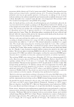
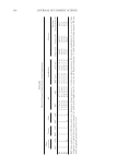
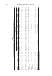
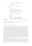
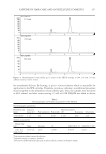
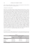
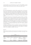
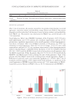
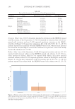
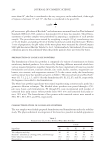
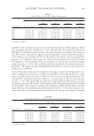
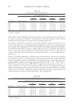
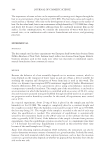
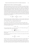
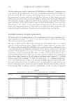
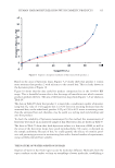
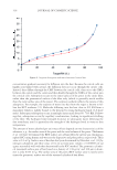
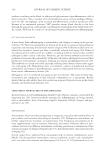
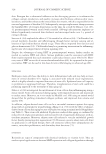
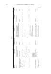
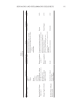
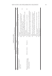
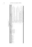
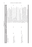
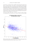
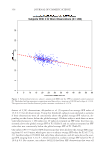
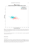
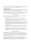
SUNSCREEN TESTING BIAS 353 would infl uence the validity of a clinical trial to determine the SPF of a sunscreen (e.g., higher SPF values obtained). Subversion bias would occur if subjects who be- come known for always generating a low SPF value for the test sunscreen are ex- cluded from future clinical trials. Similarly, subjects who become known for always generating a high SPF value might be asked to be on clinical trials. Because of the volume of observations in the data reported by Alejandria et al. (5), one might be able to discern if such individuals existed. MATER IALS AND METHODS STUDY DESIGN The 2 ,503 observations (n = 652 subjects) depicted in Figure 1 (5) were analyzed for multiple observations on the same subject. After including only those subjects with three or more observations each, the resulting subset of data (Figure 2) consisted of 2,033 observations encompassing 286 subjects (average of seven observations per subject). The average of all observations for each of the 286 subjects’ unprotected MEDs and corresponding SPF values was calculated to provide a single data point for each subject. The relationship of unprotected MED and corresponding SPF was statis- tically explored in this dataset. STATI STICAL ANALYSIS To te st if the consolidation of the 2,033 observations across subjects reduced any statistical power or changed the conclusions reported on the original dataset of 2,503 observations, a linear regression and correlation analysis were performed using the same parameters presented in Alejandria et al. (5). To te st for any patterns in the data, a k-means cluster analysis approach was used (6). The goal of the cluster analysis Figure 2. Study design.

JOURNAL OF COSMETIC SCIENCE 354 was to group the 286 subjects into specifi c partitions based on their unprotected MED and SPF values. Only similar subjects would be present within each partition (also called a cluster), and subjects from each partition would have statistically sig- nifi cant different MED and SPF values versus subjects from different partitions. To pr oduce the clusters, the following steps were performed: Step 1: Specify the numbers of clusters k. Randomly choose k subjects and declare them as the centers of each of the k clusters. These centers are also known as “centroids,” and the value of each centroid is the average of all subjects (based on their unprotected MED and SPF values) within that specifi c cluster. Step 2: Calculate the distance metric between each cluster centroid and all other data points (i.e., all other subjects) within the data set. The distance metric is the Euclidean distance between two vectors in a Euclidean space, with each vector representing a unique subject. Step 3: Assign each subject to the cluster centroid whose distance metric is the least of all the cluster centroids. Each subject should be assigned to exactly one of the k clusters, and no subject should share multiple clusters. Step 4: With all subjects now inside the k clusters, recalculate the new cluster centroids by calculating the average of all subjects within each cluster. Step 5: Repeat steps 2–4, now with a newly calculated cluster centroid for each cluster. Repeat this process until the cluster centroids remain unchanged despite further iterations. When this occurs, no more subjects should be reassigned to a new cluster. Step 1 of the k-means cluster analysis required a prespecifi ed value for the number of clus- ters k. Rather than selecting an arbitrary value, an optimal value for k was determined using the silhouette method (7). This method examined a range of possible values for k. For each of these possible values, an average silhouette width was calculated. The value of k with the largest average silhouette width was selected as the optimal cluster size for the analysis. To ca lculate the average silhouette width, the following steps were performed: Step 1: Perform the k-means cluster analysis for each of the possible values of k. A range of 1–10 clusters was tested. Step 2: Select a subject within one of the k clusters. Any subject within the cluster can be used as a starting point. Step 3: Calculate the average distance metric between the selected subject and all other subjects within the cluster. This will be the within-cluster distance. Step 4: Calculate the average distance metric between the selected subject and all subjects in a neighboring cluster. This will be the between-cluster distance. If there is more than one neighboring cluster, calculate the between-cluster distance for the remaining clusters. Step 5: Compare the within-cluster distance (Step 3) with the smallest between-cluster distance (Step 4). Calculate the difference between the two values, and then divide the difference by the largest of the two values. This will produce the silhouette width, with a value ranging from –1 to 1. Step 6: Repeat steps 2–5 by selecting another subject within the same cluster mentioned in step 2. This process will repeat until all subjects within the cluster are selected. Step 7: Calculate the average of all silhouette widths that were calculated in step 6. This is the average silhouette width for the cluster value k. If th e clustering algorithm performed well, the within-cluster distance will be small and the between-cluster distance will be large. An average silhouette width of 1 will indicate