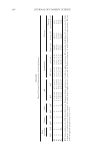
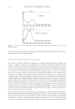
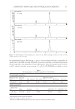
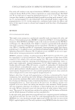
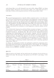
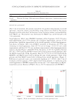
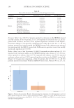
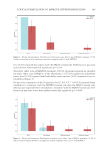
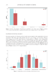
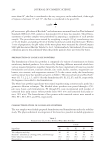
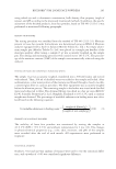
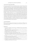
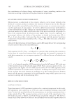
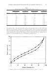
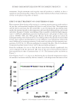
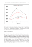
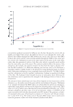
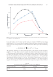
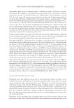
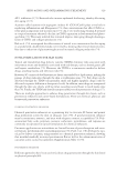
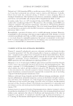
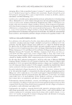
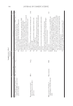
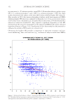
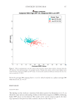
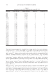
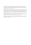
SUNSCREEN TESTING BIAS 355 the most appropriate clustering, and an average silhouette width of –1 will indicate the poorest clustering performance. After the k-means cluster analysis partitioned each subject into specifi c groups, descrip- tive statistics were calculated within each cluster. In addition, hypothesis testing using Welch’s unequal variance t-test was performed to test for any statistically signifi cant dif- ferences between the clusters. Statistical signifi cance was achieved at the 95% confi dence level (p 0.050). Finally, subjects with extreme SPF values were evaluated within each cluster and reported. STATI STICAL SOFTWARE Stati stical software R (version 3.6.1 for Microsoft Windows R Foundation for Statistical Computing, Vienna, Austria) was used for all data analyses (8). In addition to the base package preinstalled with software, the packages “tidyverse,” “cluster,” “factoextra,” and “ggplot2” were also used for the cluster analysis and for graphical plots. RESUL TS SELEC TION BIAS Aleja ndria et al. (5) reported Pearson’s product-moment correlation coeffi cient of –0.409 when evaluating the relationship between an observation’s unprotected MED value and the resulting SPF value (n = 2,503) (Figure 1). In addition, the trend line from the regres- sion analysis had an intercept of 18.579 and a slope of –0.155. By comparison, the cor- relation coeffi cient of the subject-specifi c data (n = 286 subjects) revealed a correlation coeffi cient of –0.478, and the trend line from the regression analysis revealed an intercept of 18.098 and a slope of –0.116 (Figure 3). Befor e performing the k-means cluster analysis, the silhouette method calculated 10 average silhouette widths, one for each of the possible values of k. The average silhouette widths ranged from 0.000 to 0.395. The largest average width of 0.395 was associated with a cluster size of 2, and the second largest average width of 0.341 was associated with a cluster size of 6. Using the optimal cluster amount suggested by the silhouette method, the k-means cluster analysis revealed two groups of subjects sharing similar unprotected MED and SPF values. These two clusters—labeled as “high SPF” and “low SPF”—had sample sizes of 153 and 133, respectively (Figure 4). When comparing the two clusters, the “high SPF” cluster revealed a statistically signifi cantly greater average SPF value (as well as a lower average unprotected MED value) than the “low SPF” cluster (p 0.001). For the “high SPF” cluster, the average SPF value was 16.314 and the average unprotected MED value was 18.366. For the “low SPF” cluster, the average SPF value was 14.708 and the average unprotected MED value was 25.671. SUBVE RSION BIAS To fu rther characterize the potential impact of a subject’s MED response on SPF results, subjects with extreme SPF values were evaluated within each cluster. In the original

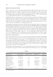
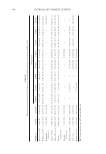
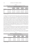
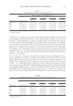
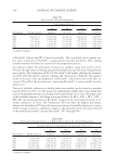
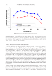
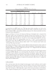
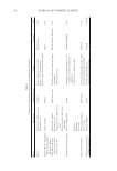
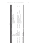
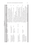
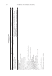
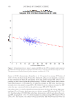
JOURNAL OF COSMETIC SCIENCE 356 dataset of 2,503 observations, Alejandria et al. (5) reported an average SPF value of 15.6 ± 2.5 for all observations. Using this threshold, subjects were declared as extreme if their observations were all consistently above the global average SPF value (or, de- pending on the cluster, below the global average). Of those subjects with three or more valid observations (n = 286 subjects), 29 subjects returned an SPF value that was con- sistently above the global average SPF of P2 (Table I) and six subjects returned an SPF value that was consistently below the global average SPF of P2 (Table II). One sub ject (#53777) had 10 SPF observations that were all above the average SPF, rang- ing from 0.5 to 6.0 units, which gave rise to a subject average SPF value for P2 of 17.5 ± 2.0. Another subject (#81609) had only three observations, and all were above the aver- age SPF, ranging from 3.2 to 4.7, which resulted in a subject average SPF value for P2 of 19.8 ± 0.9. By contrast, one subject (#61224) had four SPF observations that were all Figure 3 . Relationship between a subject’s unprotected MED and the SPF for standard control sunscreen P2. The dashed red line represents a regression trend line with a y intercept of 18.098 and a slope of -0.116. The regression trend line has Pearson’s product moment correlation of -0.478.