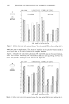
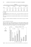
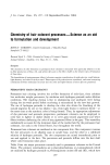
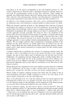
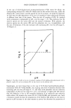
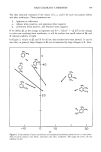
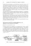
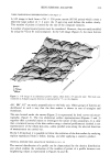
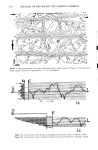
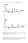
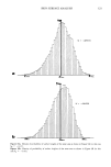
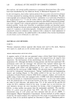
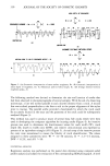
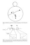
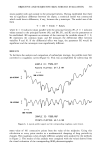
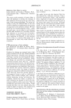
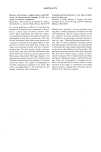
314 JOURNAL OF THE SOCIETY OF COSMETIC CHEMISTS Figure 5. Microcartography of the same abdominal positive replica shown in Figure 2. The body axis 0- degree angular direction is represented by • x in the diagram. N, Z max Z1 z Figure 4a. Construction of the density of probability function p(z) from a schematic profile. Figure 4b. Construction of the cumulative distribution function P(z) from a schematic profile.

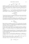
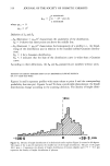
SKIN SURFACE ANALYSIS 315 Prob (z z(x) z + Az) p(z) = Lira Az--•0 Az In Figure 4a, an example of a skin surface profile is shown. Heights (z) of equidistant points are separated by intervals of Ax. The values of z are included between two extreme values (z minimum and z maximum). This interval (z maximum minus z minimum) is divided into a selected number of divisions (in Figure 4a, there are 23 divisions). The probability, p (z = z•), used for finding an experimental point with a height included between z• and z• 4- Az, is given by the ratio of the number of experimental points of height z• to the total number of points. In Figure 4a, p (z = z•) = 6/N, z maximum with fp(z) dz = 1 z minimum The last formula shows that the probability of finding a point, which is situated between z minimum and z maximum, is equal to one (as any point is located between extreme values z minimum and z maximum). In the same way, the probability of finding a point at a height inferior to z is given by the distribution function (accumulated frequencies) which gives the number of points located between the minimum value and a given value z•l, as shown in Figure 4b. f z(1) P(z) = p(z) dz z minimum Figure 4b shows the construction of the P(z) curve. The lowest points of the profile are located at z minimum. The number of points is the number between this minimum value and any value zl (i.e., the experimental points distributed in the lined area are given by P(zl)). In this example P(zl) = 7/N. Successive moments of the distribution p(z), especially the central ones, in relation to the mean value • of heights, allow the classical roughness parameters (Ra, Rp, Rmax, Rtm, etc) (13) and statistical parameters, such as standard deviation (g), to be deter- mined. It is evident that either of the parameters cr or cr 2 and the mean value • are sufficient to describe the height distribution according to the Gaussian distribution. We used the central moments [xo• and [x•4 • of height distribution (or slopes and curvatures) in relation to the mean value. In Figure 4a, there are nl points which have heights equal to Zl therefore p(z•) = n•/N (with N equal to the total number of points of the profile, and in this example, nl = 6). Each of these points, having a height, z, is given a coefficient equal to the distance separating each point from the mean value of the profile (i.e., d = z - •). The moment of order n of the profile is given by the sum of the terms: • nl --(z - •) where,= p(z)