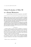
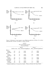
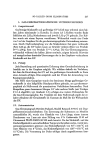
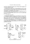
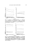
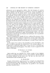
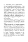
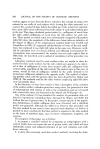
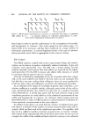
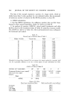
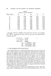
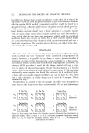
9.60 JOURNAL OF THE SOCIETY OF COSMETIC CHEMISTS S 1 S 2 S 3 S 4 Sn- 1 S n T1 T2 T1 T2 t t T1 T2 T 2 T 1 T 2 T 1 T 2 T 1 A 1 A 2 Figure 1. SSEM design represented as a crossover: As represents left axillae Aa represents right axillae Sa, Sa . . . S,• represent subjects T• represents antiperspirant Ta repre- sents control. (Appropriate randomization not shown.) tions begin in order to provide conformance to the assumptions of normality and homogeneity of variance. (The work reported in the earlier paper (5) showed this to be necessary, and has been confirmed by a large number of subsequent experiments. ) A second important feature is the type of randomi- zation procedure used, which is appropriate to the crossover design. RM Analysis The SSEM analysis, coupled with correct experimental design and random- ization, can be shown to produce statistically unbiased estimates of per cent reduction and experimental error. The RM uses a similar design, but the analysis normally used assumes that sides effects are removed by the adjust- ment procedure. For the RM to remove side effects fully, however, it would be necessary that the pretest ratios be constants. It is easy to observe by examination of any set of pretest ratios done repeat- edly on the same subjects (see Table I) that the ratios are not constants. The [act that they are more uniform than milligram values of sweat produced is irrelevant, since ratios, not milligrams, are used in the adjustment procedure. As an indicator of the degree of variability of pretest ratios w/th time, a cor- relation coefficient is a suitable statistic, although certain kinds of bias will re- main undetected thereby. We carried out such tests on a number of pretest ratios determined 1, 3, and 21 days apart with the same subjects, using a rank correlation procedure to avoid violation of the statistical requirements of nor- mality and homogeneity of variance. We obtained values ranging from less than 0.50 to 0.87 (a value of 1.00 would have indicated perfect correlation be- tween successive measurements on the same subjects). In addition to the above, we noted that the variance of adjusted mean post- test ratios is a function of the number of pretest measurements made and av- eraged, which are then used in the adjustment procedure. It is possible, with the use of_ a_ sufficient number of pretest measurements, to exercise consider- able control of the experimental error of the final mean ratios. In one case, for example, the width of the confidence limits about the mean per cent reduction

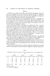
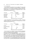
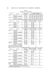
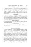
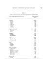
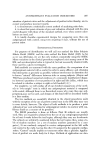
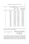
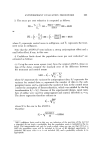
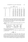
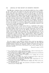
ANTIPERSPIRANT EVALUATION PROCEDURES 261 Table I Typical Set of Txvo-Sample Test Data: Pad B Only, Four Applications before Posttest Readings (Milligrams and Ratios) Subject Number Treatment On (side) PRETEST DATA POSTTEST DATA Day 1 Day 2 (after 4 applications) Ri'ght Left Right Left Right Left 13 R (mg) 606 599 690 704 263 630 (ratio) 1.012 0.980 0.417 14 R (mg) 657 606 776 695 445 670 (ratio) 1.084 1.117 0.664 15 R (mg) 630 555 646 593 304 380 (ratio) 1.135 1.089 0.800 16 R (mg) 356 262 415 310 217 420 (ratio) 1.359 1.339 0.517 17 R (mg) 400 409 489 546 336 497 (ratio) 0.978 0.896 0.676 18 R (mg) 210 350 394 556 288 557 (ratio) 0.600 0.709 0.517 19 L (mg) 789 332 1060 809 850 365 (ratio) 0.421 0.763 0.429 20 L (mg) 710 589 750 568 400 257 (ratio) 0.830 0.757 0.643 21 L (mg) 725 607 825 684 460 261 (ratio) 0.837 0.829 0.567 22 L (mg) 809 663 312 243 430 200 (ratio) 0.820 0.779 0.465 23 L (mg) 587 612 745 860 788 325 (ratio) 1.043 1.154 0.412 24 L (mg) 618 461 547 523 555 283 (ratio) 0.746 0.956 0.510 varied, as the number of pretest measurements used to compute a geometric mean pretest ratio was increased, as follows: Number of Pretest Measurements Width of 95% CL about Per Cent Reduction Computed From Adjusted Posttest Ratios 26.4 (% reduction units) 22.6 (% reduction units) 17.2 (% reduction units) This reduction of the confidence limits about the PR is sufficient so that, even with geometric means of only two pretest ratios, it is often possible to equal or exceed the prec sion obtained with the SSEM when a single posttest determination is used with the latter. This was the case in examples 2, 3, 4, and 5 of Table VII (as will be shown later). Of course, the precision of the SSEM