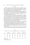
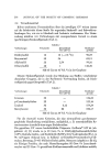
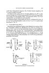
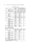
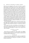
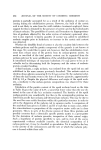
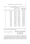
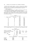
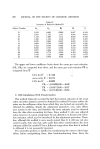
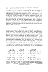
268 JOURNAL OF THE SOCIETY OF COSMETIC CHEMISTS Table IV Summary of Ratios for Method B -- Subject Number Rp• Rpo. tl•, lit 13 1.012 0.980 0.996 0.417 0.419 14 1.084 1.117 1.101 0.664 0.603 15 1.135 1.089 1.112 0.800 0.719 16 1.359 1.339 1.349 0.517 0.383 17 0.978 0.896 0.937 0.676 0.72I 18 0.600 0.709 0.655 0.517 0.790 19 0.421 0.763 0.592 0.429 0.725 20 0.830 0.757 0.794 0.643 0.810 21 0.837 0.829 0.833 0.567 0.681 22 0.820 0.779 0.800 0.465 0.582 23 1.043 1.154 1.099 0.412 0.375 24 0.746 0.956 0.851 0.510 0.599 The upper and lower confidence limits about the mean per cent reduction (PR1, PR•,) are computed from these, and the mean per cent reduction PR is computed from R' -- UCL for R' = 0.7146 mean ratio, R' = 0.6173 LCL for R' = 0'.5200 PR1 = (1-0.5200) 100 = 48.00 '•: PR = (1-0.6173)100 = 38.27 PRa = (1-0.7146)100 = 28.54 ß , C. BM Calculations With Transformation This method takes into account the fact that correct estimates of the mean ratios and other statistics cannot be obtained by method B because neither the ratios nor the milligram values from which they are derived are normally dis- tributed. In addition, despite the adjustment procedure, some sides effects may remain in the data, and therefore the error estimate must be obtained from the data after accounting for these. Since method C also uses adjusted ratios, however, it cannot compensate for any distortion in the per cent reduc- tion estimates , which may be introduced by the adjustment procedure. There- fore, although the method is more nearly Correct than B, it still may not give correct results. Note also that, quite aside frbm these considerations, the error estimate yielded by method C has a different composition than that of method A, although it is not necessarily incorrect. The normality problem is handled by transforming the ratios to their loga- rithms before manipulating them, then back-transforming them. Since the

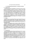
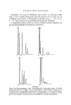
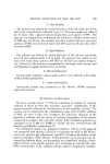
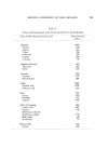
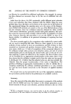
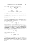
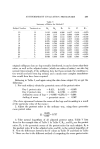
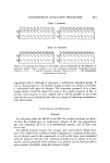
ANTIPERSPIRANT EVALUATION PROCEDURES Table V Summary of Ratios for Method C 269 Subject Number Treatment on 13 R 1.019. 0.980 0.996 0.417 0.419 --0.870 14 R 1.084 1.117 1.100 0.664 0.604 --0.504 15 R 1.135 1.089 1.112 0.800 0.719 --0.330 16 R 1.359 1.339 1.349 0.517 0.383 --0.960 17 R 0.978 0.896 0.936 0.676 0.722 --0.326 18 R 0.600 0.709 0.652 0.517 0.793 --0.232 19 L 0.421 0.763 0.567 0.429 0.757 --0.278 20 L 0.830 0.757 0.793 0.643 0.811 --0.209 21 L 0.837 0.829 0.833 0.567 0.681 --0.384 22 L 0.820 0.779 0.799 0.465 0.582 --0.541 23 L 1.043 1.154 1.097 0.419. 0.376 --0.978 24 L 0.746 0.956 0.844 0.510 0.604 --0.504 original milligram data are log normally distributed, it can be shown that their ratios, as well as the adjusted ratios (which are ratios of ratios) are also log normal. Interestingly, if the milligram data had been normal, the resulting ra- tios would not have been log normal, and a much more complex transforma- tion would then have been required. Referring to Table I, and again using the data fr'om subject 19, we get the following: 1. For each subject, obtain the geometric mean of the pretest ratios Day 1 pretest ratio = 0.421 In 0.421 =-0.865 Day 2 pretest ratio = 0.763 In 0.763 ---- -0.270 Arithmetic mean of logs = (-0.865 -0.270)/2 = -0.568 Antilog of mean = geometric mean -- 0.567 (The close agreement between the mean of the logs and its antilog is a result of the particular value of the mean.) 2. Adjust the posttest ratios in the ordinary way, using these geometric mean pretest ratios 0.429 R-• =0.•= 0.757 3. Take natural logarithms of all adjusted posttest ratios. Table V lists these for the example data of Table I. In Table V, Rp•, and Rp2 are the pretest __ ratios RG is the geometric means of the pretest ratios for each subject Rt is the posttest ratio R' is the adjusted ratio and R'•, is the natural logarithm of R'. Note the differences between the R' values in Table IV and those in Table V. These are due to the different method of computing the mean pretest ratio.