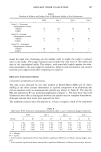
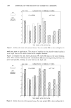
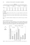
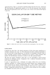
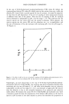
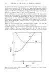
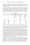
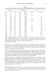
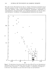
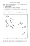
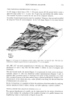
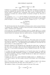
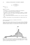
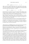
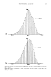
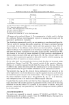
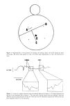
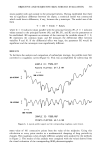
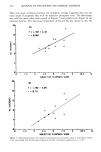
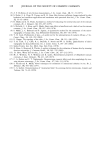
SKIN SURFACE ANALYSIS 313 THREE-DIMENSIONAL REPRESENTATION (3-D) (Figure 2) A 3-D image is built from a 256 X 256 point matrix (65536 points) which covers a relatively large surface (4 X 4 mm). the 15-•m step used defines the surface clearly. This number of points is limited by the size of the computer memory. A number of experimental points must be considered. However, they are easily satisfied by using the Victor S 1 microcomputer. In the 3-D image (Figure 2), the main furrows 200p m OOpm 200pro Figure 2. 3-D image of an abdominal positive replica taken from a 55-year-old male. The body ax•s considered as O-degree angular direction is represented by --• x in the diagram. AA', BB', CC' are nearly perpendicular to the body axis. Other groups of furrows are distributed in such a way that the skin surface is shown in sets of triangles and rhombuses. The area located under the arrows (Figure 2) is represented by level curves (microcar- tography, Figure 3). The two abdominal surface representations (Figures 2 and 3) together offer a powerful means to investigate the nature of skin anisotropy. It is clear that a statistical survey of the skin surface using a classical profilometric method is not representative of the whole skin area, unless parallel scans along the selected direction of measurement are carried out. By the 3-D method, it is possible to follow the evolution of the skin surface by studying replicas reproduced from it before, during, and after applying a cosmetic product. VERTICAL DISTRIBUTION ANALYSIS OF PROFILES (9,10,11,12) The vertical distribution of a profile can be characterized by the density distribution p(z) which enables the evaluation of the number of points of a profile between two neighboring values as represented in Figures 4a and 4b.

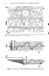
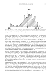
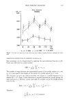
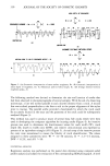
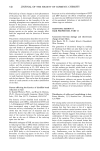
314 JOURNAL OF THE SOCIETY OF COSMETIC CHEMISTS Figure 5. Microcartography of the same abdominal positive replica shown in Figure 2. The body axis 0- degree angular direction is represented by • x in the diagram. N, Z max Z1 z Figure 4a. Construction of the density of probability function p(z) from a schematic profile. Figure 4b. Construction of the cumulative distribution function P(z) from a schematic profile.
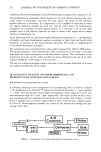
Purchased for the exclusive use of nofirst nolast (unknown)
From: SCC Media Library & Resource Center (library.scconline.org)