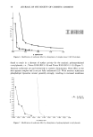
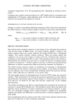
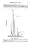
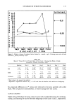
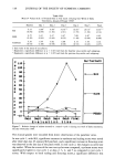
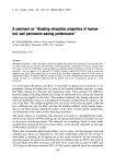
74 JOURNAL OF THE SOCIETY OF COSMETIC CHEMISTS Figure 2. Set-up for fluorescence measurement and computer monitoring. Determination of organic phosphate. The surfactant interacts with the phospholipid in a direct molar ratio. To standardize the phospholipid aliquot the organic phosphate concentration of the liposomes was determined by the method of Stewart (18). Liposome working aliquots were calculated so that the final concentration in the test solution was 0.05 mM phospholipid. Monitoring the release of carboxyfluorescein from liposomes. Maximal potential fluorescence (100%) was determined by destroying a working aliquot of liposomes in a 10-mM solution of taurodeoxycholate. For the 0% value, the fluorescence intensity of a liposome working aliquot in isotonic 0.05-M Tris buffer was established. Leakage of marker from liposomes in buffer was negligible over the course of several hours. In a method previ- ously developed for the study of bile acids (19), a constant amount of liposomes (see above) was added to an isotonic test solution containing surfactant, so that the final volume was 4 ml. After mixing, solutions were quickly transferred to Ultra-Vu poly- propylene disposable cuvettes (American Scientific Products) and placed into the fluo- rimeter that was interfaced with an IBM personal computer. A computer program was developed that recorded fluorescence values at regular time intervals and also the time (in minutes) at which 50% of the maximal fluorescence was read. This point was identified as t«. The readings can, however, be recorded quite easily with a stopwatch. Interpretation of d•ta. The effect of each surfactant on the liposomal membranes was determined over a wide concentration range. For each concentration the t« value was established. Plots of t V2 vs surfactant concentration yield curves that are indicative of the way in which each surfactant interacts with the liposomal membranes. (Figures 4-12). As the surfactant monomer concentration increases, the t« value decreases. In the region of the CMC, the monomer concentration stabilizes and with it the t« value. The CMC, therefore, can be recognized as the "bend" in the curve. It is well known that the individual surfactant molecules are the irritancy-producing

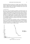
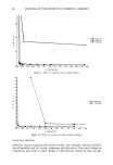
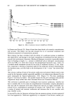
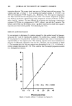
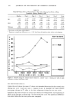
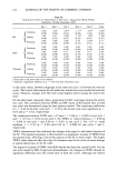
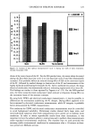
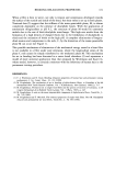
SURFACTANT-SKIN INTERACTIONS 75 species of a surfactant system (9), especially for the liposome model. Micelies may, however, be involved in producing irritation in the soap chamber test, as little is known about the actual interactions taking place between surfactant solutions and the skin during prolonged exposure (20,21). Development of a numerical irritancy index. The exponential functions obtained from the "concentration vs tV2" plots showed that the milder surfactants usually result in a curve that is less tightly bent. 'With a computerized curve-fitting program, the function y = a + b*exp (- c'x) was found to fit the available data most closely (Figure 3). The absolute value of ( - c), when placed in rank order, showed an increasing "c-value" with increasing irritancy (Table I) for a group of anionic surfactants and blends. A reasonable rank correlation was observed between most "c-values" and numerical soap chamber scores (Toxicol, U.K.) of the same surfactants (Figure 13). The correlation does not exist for nonionic surfactants. The results also demonstrate the problems associated with the assessment of irritancy by a test panel. The soap chamber data were obtained in two separate runs several months apart. ALS and SLS were the most irritating surfactant in each run. Each received the score of 4.75. This clearly demonstrates the importance of including the same standard with every batch of compounds to be tested that runs counter to the need to keep expenses low. RESULTS It was important to demonstrate that the described method is sensitive enough to rank the irritancy of most of the surfactants tested, ideally in the same order as the soap chamber tests. The rank correlation was found to be good for a series of anionic surfactants. With these surfactants, the method was found sensitive enough to respond 5. O"T : : .. :.. '"i ............. *'x .... =================================== o., l W.. ............................ • ......... ß ............ . ......... ß ..... o.o I I I --3----3-----3-- • ! •- I I -I - 0.00 0.02 0.04 0.08 0.08 O.iO 0.t2 0.t4 0.t8 0.t8 0.20 0.22 0.24 • suPfsctsnt • SLS:O.28+43.93•exp(-127.56•x) ß SLES-coco:O.6+lS.06•exp(-32.08•x) ß SLES-oxo:O.59+4.45•exp(-47.86•x) ß SLEC:O.71+13.98•exp(-21.19•x) Figure 3. Example of curve fittings If(x)= a+ b*exp(- c*x)].