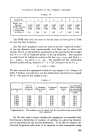
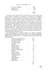
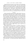
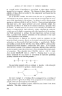
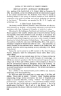
JOURNAL OF THE SOCIETY OF COSMETIC CHEMISTS diameter, ED50, which, as the distribution is symmetrical, is also the diameter either side of which lie 50 per cent of the particles. We can also ' obtain an estimate of s, the estimated •, this being the diameter at 84.13 per cent, divided by that at 50 per cent. Divided, because the diameter scale is logarithmic and subtraction of the length of the scale at 50 per cent from that at 84.13 per cent is equivalent to division of the numerical value of the diameter at the one point by that at the other. Our results are: TABLE II Sample No. 1 2 3 4 5 6 7 ED50, microns 1.40 1.47 2.23 2.04 1.40 2.70 2.95 s microns 5.6 3.7 3.7 2.6 5.6 3.0 2.0 It is apparent that it is worth while to analyse the data in more detail and the appropriate first steps are ß (i) Convert the "cumulative percentages smaller" to probits (the probits directly derived from the data are called "empirical probits," tables of which are in most books of statistics, e.g., Refs. 10 and 13) and the diameter of the largest particles in any group to log microns. This gives: TABLE III Empirical probit of cumulative % smaller Log•0 microns 1 2 3 4 5 6 7 0.279 5.21 5.10 4.80 4.91 5-18 4.68 4.28 0.591 5.80 5.76 5.42 5.69 5.83 5.30 5.45 0.771 6.00 6.05 5.72 6.06 6.03 5.65 6.06 0.898 6.19 6.25 5.92 6-32 6.17 5.95 6.41 0.996 6.33 6.41 6.08 6.55 6.30 6.17 6.68 1.076 6.42 6.51 6.21 6.66 6.42 6.30 6.76 (ii) These empirical probits are now plotted on arithmetical graph paper and the best fitting line drawn to them by eye. In fitting this line to the points, attention should be paid to placing it so that on one side of the line the sum of the differences, in probits, of the points and the line, at the same log diameter, is the same as the sum of those on the other side of the line. The appropriate lines for emulsions Nos. 3 and 4 are shown in Graph 2. As described in Part II (ii), they can be used to provide estimates of ED50 and of s. They give: 162

STATISTICAL METHODS IN THE COSMETIC INDUSTRY TABLE IV Sample No. 1 2 3 4 5 6 7 ED50, Log Microns 0.106 0.204 0.366 0.260 0.095 0.435 0.463 ED50, Microns 1.26 1.60 2.32 1.82 1.24 2.72 2.90 s, Log basis 0.654 0.538 0.582 0.485 0.675 0.538 0.318 s, comparable to Table II 4.5 3.45 3-• 3.05 4.7 3.45 2-08 The ED50 value and s are more or less the same as those given in Table II, but note that in micron. (iii) The above graphical results are used to provide "expected probits" at the log diameter used experimentally, and these can be either read directly from it or calculated by substitution in the equation for the straight line Y = a + bX (Y being the probit, X the log diameter). This equation is easily found by taking two points on the line, x•ya x,y,, and then b ---- (y•--y,)/(x•- x,) and a--y•- bx•. The equation for the relationship between probit and log. diameter, Y ----- a q- bX, is found to be for No. 3: Y ---- 4.37 q- 1.72X. We have entered the appropriate results for the sample 3 in Column 5 of Table V (below), and will carry out the arithmetical calculations for Sample No. 3. Our data for this sample is now: TABLE V No. of % particles particles % Particles Empirical Expected below stated Log diameter examined below stated probit probit. size calculated .¾ * size Y from expected probit 0.279 2,000 42.2 4.80 4.85 44.0 0.591 2,000 66.2 5.42 5.39 65.2 0'771 2,000 76'3 5-72 5'71 76.1 0.898 2,000 82.2 5.92 5.91 81.9 0.996 2,000 86-0 6.08 6.08 86.0 1.076 2,000 88-7 6.21 6.23 89.1 * Approximately. The numbers are not stated, bug the text states that around 2,000 were measured. (iv) We also want to know whether the assumption is reasonable that the frequency distribution of numbers of particles at a given log diameter can be represented by the normal distribution. To do this we compare the observed frequencies with those to be expected on that assumption, using 163