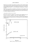
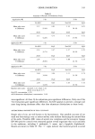
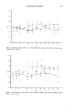
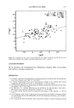
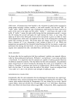
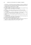
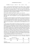
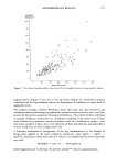
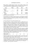
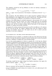
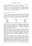
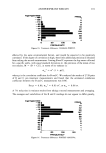
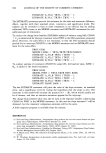
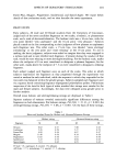
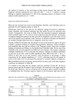
176 JOURNAL OF THE SOCIETY OF COSMETIC CHEMISTS Log Standard Deviation 0.35 0.30 + 0,25 0.20 0.15 + A A A A A A A A A A A A A A A A A A A A A A A A A A AA A A A A AA AA A A A A A A B A B A A A A A A A A A B A A AA A AA A A A A AA AA A A AA A AA AB A A A AA A A A A AA AA A BA A A AAA A A A AA A A AA A B A A A A AA A AA A B A 0.1.0 + A A A A A A A A A 0.05 Log Mean Sveat Rate Figure 6. Test subject baseline axillary log(sweat rates): Plot of standard deviation versus mean by subject. THE POSTRT MODEL FOR ANALYSIS OF POST-TREATMENT DATA Further consideration of the experimental design leads to an extension of the SSEM model. The assignment of treatments to experimental units is made in such a way that each treatment is applied to the left axilla for half the subjects and to the right axilla for the other half. Subjects are randomly placed in one of two groups: those having treat- ment "T" on the left and "C" on the right (Group 1), and those with the opposite assignment (Group 2). Subjects may be considered as larger experimental units assigned to one of the two levels of a factor called "groups." Axillae may be considered as smaller experimental units assigned a value of each of the two factors, "sides" and "treatments." In statistical parlance this is a "split plot" design, i.e., there is more than one size of experimental units, with units of each size assigned to levels of different sets of factors. Since subjects are randomly assigned to groups, any difference in group means should be subject only to random chance, with an expected value of zero. However, the "groups" factor is aliased with the treatment-sides interaction. If the interaction exists, it leads to the conclusion that the comparative efficacy of two treatments depends upon which side of the body the test treatment is applied. It is important to note that this interaction effect must be tested against main plot error, which is the variation due to subject differences in mean sweat rate.

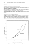
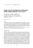
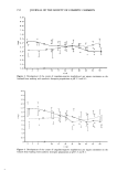
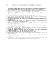
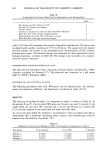
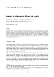
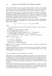
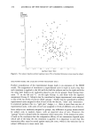
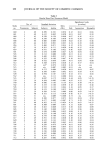
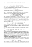
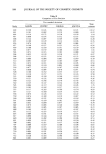
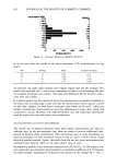
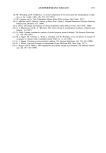
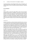
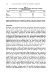
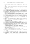
ANTIPERSPIRANT RESULTS 177 Standard Deviation 0.8 0.7+ 0.6+ 0.5+ 0.4+ 0,3+ 0.2+ 0.1 0.0+ i A A B A A AA AA A AA A A A A A A A A AA AA ABAB AA A A A A AABA A AA A AB CC A A A B AC ABAAB A A ACAB C ABAAAB A AA AA B •B A ABABA A A ABA CAAA B C A A A A A BA AA A A A A A A A A 0,6 0 1.0 1.2 1.4 1.6 Mean Sweat Ratio Figure 7. Test subject baseline axillary right/left sweat ratios: Plot of standard deviation versus mean by subject. Given this interpretation of the experimental design, a more explicit mathematical model is available to describe the relationship of the response to the experimental factors. This model, which we shall call the post-treatment (POSTRT) model, is as follows: Yijkm = •-m-'Yi -m- •j(i) -m- )k k "{- "r m "{- ejkm(i) where: Yijkm is the logarithm of the sweat rate for axilla k of subject j in group i, treated with treatment m is the log mean sweat rate over all subjects and axillae is the fixed effect of groupi, i = 1 (k = m), 2 (k • m) 0j(i) is the random effect of subject j nested in group i, j = 1, 2, . .., ni, the parentheses denoting nesting is the fixed effect of side (laterality) k, k = 1,2 (left, right) m is the fixed effect of treatment m, m = 1,2 (control, test) oejkm(i) is the random effect of axilla k of subject j nested in group i treated with treatment m. subject to: Z•/i = 0, •)k k = 0, •'r m = 0 i= 1,2 k= 1,2 m= 1,2 0ii) is N (0, eL2), independent for all i, j,