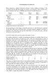
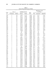
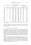
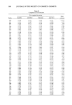
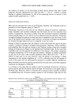
182 JOURNAL OF THE SOCIETY OF COSMETIC CHEMISTS Table I also lists results of normality tests that were performed on the residuals (observed minus predicted log sweat rates). These results showed significant departure from normality in only three studies, which lent additional support to the use of the loga- rithmic transformation of the data. The normality tests used were the Shapiro-Wilk test for 50 subjects or less, and the Kolmogoroff-Smirnoff test for greater than 50 subjects. The sides by treatment interaction effect was rarely significant at the 0.05 level, oc- curring in only two studies. These results demonstrate that the interaction effect is negligible. The main plot analysis can therefore be dropped from the analysis, as its only purpose is to test this interaction. Note that if the interaction mean square were mistakenly tested with the split plot error term, instead of the main plot error term, the incidence of "significant" results would greatly increase, giving rise to erroneous con- clusions. A SIMPLER MODEL FOR POST-TREATMENT DATA ANALYSIS Since the treatment by side interaction is nonexistent, the main plot analysis is no longer of interest, and only the split plot analysis need be considered. The split plot analysis is essentially an analysis of the log(R/L) ratios or, equivalently, the differences of the log sweat rates within subjects. To develop the model, consider the two-treatment case where the log ratio of the post- treatment sweat output of right to left axillae, log(R/L) = log(R) - log(L), is: Pij = Yij2m -- Yijlm, for subject j in group i, m • m'. Substituting for the Y terms using the POSTRT model and noting that the whole plot factor levels cancel within a given subject, the resulting model is: P•i = 0t2 - )t•) + (% -q-l) + ½P•i for subjects in group 1, and P2j = ()k2 -- )k l) -- (q-2 -- q'l) •- eP2j for subjects in group 2, where the variability terms EPlj = •j22(1) - •jll(1) and •P2j = •j21(2) -- •j12(2) are N (0, (Tp2), (Tp 2 = 2or 2. Thus the variance of the differences are twice the variance of the split plot variance cr 2. To further simplify the model, we can let )t = k 2 - )t• represent the sides effect and q- = q-2 - q-• represent the treatment effect, and write the model as: P•i = )t + q- + ½P•i for subjects in group 1, and P2j = k - q- + eP2j for subjects in group 2, IfPs. and P2. represent the mean differences over subjects in each group, then the sides effect, )t, and treatment effect, % are estimated, respectively, as: Lp = (P•. + P2.) / 2, and Tp = (PL - P2.) / 2. An estimate of crp 2 is afforded by the pooling the within-group sample variances of the Pii as follows: Sp 2 = -- P1.) + - P2.) 2 (nl • , -3- n 2 -- 2)

ANTIPERSPIRANT RESULTS 183 The confidence interval for the log difference in sweat rate between treatments is calculated as follows: Tp ñ t(l_ot/2,df) (Sp) [(1/n• + l/n2)] 1/' where t = upper 1-or/2 th percentile of the Student's t distribution with df = (n• q- n2 - 2). After calculation, the mean difference and its upper and lower confidence limits are back-transformed to the original sweat rate units of mg/20 min. Wooding and Fink- lestein (6) denoted this as Method A and presented a numerical example. A feature of the RRB design for multiple treatments is that estimates of Tp for each treatment pair come from two sources: (a) a direct estimate from the cell containing those two treatments, which is the same estimate as described above for the two- treatment case, and (b) an indirect estimate derived from pairs of cells having each treatment in common with another treatment. An example of an indirect estimate of treatments A and B is the difference in Tp between the AC cell and the BC cell. Indirect estimates have twice the variance of direct estimates and therefore require twice the sample size per cell to achieve precision equivalent to the direct comparison. USE OF BASELINE DATA--THE SIMPLE CHANGE FROM BASELINE MODEL When baseline data are available, it is desirable to make use of the information that they contain to increase the precision of the post-treatment analysis and to correct for possible bias due to imbalance in baseline R/L ratios between groups. It is true that random assignment of subjects to groups will, in the long run, balance differences in baseline R/L ratios among test groups. For any particular study, however, numerical differences in average baseline R/L ratio will always exist between groups due to measurement variation and random assignment, and the extent of these differences will vary for pairs of treatments. Since clients are only concerned with their study, not the long run, they are typically interested in checking for baseline differences and in making corrections where these differences occur. Earlier practitioners have been concerned about this and have suggested corrections for baseline effects. The form of baseline correction cited by Majors and Wild (4) was to divide the subject's right/left axillar post-treatment sweat ratio (Rp/Lp) by the corre- sponding right/left axillar baseline sweat ratio (Rb/Lb), resulting in a ratio of ratios. In the log metric this becomes a subtraction process, which is derived as follows: 1og{(Rp/Lp)/(Rb/Lb) } = log(Rp/Lp) - 1og(Rb/L b) = {1og(1 v) - log(L)}- {1og(10 - log(L0}. To develop a model for this simple change from baseline adjustment, first equate the baseline response, 1og(R b) - log(Lb), as: Bij = Yii• - Yii•' for subject j in group i, (Since no treatment has been applied the subscript m vanishes.) Using the POSTRT full model without the treatment term, and substituting for the Y's, the model becomes: