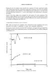
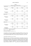
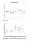
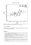
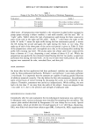
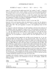
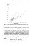
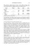
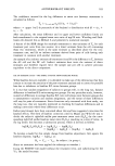
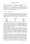
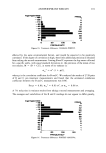
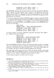
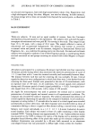
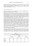
192 JOURNAL OF THE SOCIETY OF COSMETIC CHEMISTS --12 0 o FREQUENCY Figure 15. Treatment differences: CHGBAS-ANCOVA. 1 4, 174, •o 6 4, 1 2 as can be seen from the results of the above-mentioned 2728 measurements (in log units): Side Reading Mean Standard deviation R B 2.62 0.31 R C 2.64 0.27 L B 2.58 0.30 L C 2.61 0.28 As expected, the right axilla readings were slightly higher than the left readings. The results indicated that the C values were comparable in value to the B readings and that the standard deviations were similar. The right-left differences for the B and C collec- tions were also similar. It could be argued that the expense of the second measurement is minimal compared to the fixed costs of conducting a study and that the second result can be used as a check for bad data. Indeed, we have found occasional cases where the B and C collections yielded contradictory results and have used this information to reject data, using very conservative criteria. However, the tradeoff between cost and additional information must be resolved by the individual clinical laboratory. MULTIPLE BETWEEN-DAY SWEAT MEASUREMENTS The second case of repeated measures arises when repeat measurements are taken on multiple days. In the pre-treatment case, these are meant to provide additional infor- mation on baseline sweat performance. This information may, in some procedures, be used for adjustment of post-treatment values or may be used to check current versus historical panelist response. Again, the results from the two hot-room measurements are correlated since they are taken on the same subject close in time. Retrospective analysis of pre-treatment measurements, D• and D2, on 206 subjects over two consecutive pre-treatment days resulted in a correlation coefficient of 0.74 between the daily averages. Applying the formula for the variance of the average, M = (D1 q-

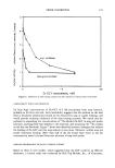
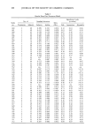
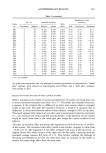
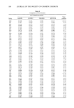
ANTIPERSPIRANT RESULTS 193 D2)/2, as in the previous section, •rm 2 = •r 2 (1 + p)/2, with p the correlation coefficient between days, we found that the variance of the averages over the two days was 0.87 of the single-day variance. However, multiple baselines can only be run at the expense of fewer treatment applications or extending the test period beyond five days. It may be more cost-effective to increase the number of panelists than to disturb the test logistics, but again this is a question that must be decided by individual circumstances. The correlation of repeated measures data appears to decrease over time. In one test with 25 subjects, seven consecutive daily pre-treatment hot-room measurements were con- ducted. The correlation coefficients of the log ratios of right over left axillae sweat rates as a function of lag time in days were as follows: Lag, days Lag correlation coefficient 1 0.71 2 0.69 3 0.69 4 0.63 5 0.59 6 0.45 The magnitude of these coefficients is in general agreement with similar work by Wooding (5), where he found correlation coefficients for pre-treatment measurements to vary in the range 0.50 to 0.87 for lag times of 1, 3, and 21 days. Multiple post-treatment measurements are different from the pre-treatment case in that each is preceded by differing numbers of treatment applications. Averaging these results is not strictly valid, since each day measures a different phenomenon. The multiple measures can be used to follow a time course, and in these cases the correlation must be taken into account in the analysis. Winer (8) outlines multivariate procedures for these repeated measures applications. TEST POWER OR THE PANEL SIZE REQUIREMENT Perhaps the most frequently asked question of a statistician is: "How many subjects do we need for this study?" To answer this question, we need to know the estimate of the test variability, usually expressed as the standard deviation, and the difference in efficacy to be detected. When the efficacy difference is expressed in terms of percent reduction, the sample size also depends on the efficacy levels. Table III has been constructed to give estimated sample sizes needed to declare two treatments significantly different at the 0.05 significance level at 80% power. The difference is specified in terms of the higher and lower percent reduction levels. By 80% power we mean that this difference would be declared statistically significant in 80% of future studies. This table is based on a standard deviation estimate of 0. ! (log units), but this value may vary for different laboratories. The sample sizes were estimated using the approximate method given by Kupper and Kafner (!5), their formula 4. General formulae can be developed to show the relationship of treatment comparison precision with panel size in multiple-treatment studies. Let n represent the number of