184 JOURNAL OF THE SOCIETY OF COSMETIC CHEMISTS Bii = k + ebii, for subjects in both groups, where k = 0% - k•), and the baseline variation •bij is N (0, trb2). If B•. and B2. are the mean baseline differences over subjects in each group, then the average baseline sides effect is estimated as: B.. = (B•. + B2. ) / 2. The simple change from baseline for each subject is the difference Cij = Pij - Bij, where Pij has previously been defined as the post-treatment sweat ratio log (Rp/Lp). Substituting for Pij and Bii , the change from baseline (CHGBAS) model is: Cli = 'r +½cti for subjects in group 1, and C2i = -'r + ½c2i for subjects in group 2, where the change from baseline variation ½•ii is N (0, ty•2), and 'r = (•2 - 'r l) is the previously defined treatment effect. There is no k term in the model, since we assume that the k terms for Pii and Bii are the same, namely the sides effect for the panel. The assumption that the k terms cancel could be questioned on the grounds that a treatment application could change the average sides effect for the panel. In this case we could represent the baseline sides effect as )kp and the post-treatment sides effect as )k b. The model would then become: Clj : ()kp -- )kb) •- 'I' -{- eclj for subjects in group 1, and C2j -- ()kp - )kb) -- 'r -t- e•2j for subjects in group 2. We have seen that the estimated value of )kp - )k b iS close to zero when averaged over the 70 past studies, and we have concluded that this difference is negligible and may be disregarded. -- -- If C•. and C2. represent the averages over groups, then the treatment effect is estimat- ed as: T• = (C•. - C2.)/2 = (P•. - P2.)/2 - (B•. -- B2.)/2 = Tp - T b -- __ where T b = (B1. - B2.)/2. Statistical calculations are then carried out as they were before for the POSTRT treat- ment effect, Tp. In the statistical literature this method is called the analysis of change (from baseline) and is discussed by Fleiss (9). Both the POSTRT (Tp) and CHGBAS (To) estimates are unbiased, i.e., both of their expected values are equal to 'r, and their difference has an expected value of zero. For any particular study, the POSTRT and CHGBAS estimates will be numerically different, since the baseline correction (Tb) is a random quantity that varies about its expected value of zero. It might be thought that the CHGBAS model will result in greater precision since it takes baseline variation into account, but this will not necessarily be so. The standard deviation of the CHGBAS model, ty• is' sqrt ((Tp 2 -t- (Tb 2 -- 2OpbO'pO'b) which is dependent on the degree of correlation of pre- and post-treatment values over subjects, measured by the correlation coefficient, Ppb- Therefore, the ratio of the baseline corrected standard deviation to the post-treatment standard deviation is:

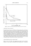
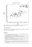
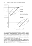
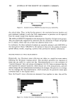
ANTIPERSPIRANT RESULTS 185 Crc/Cr p = sqrt (1 + 0 2 - 2ppt,0), where 0 = orb/or p. To achieve a reduction in variation, Ppb 0/2. If 0 is unity, for example, then Ppb must be greater than 0.5 to achieve a variance reduction via simple baseline correction. USE OF BASELINE DATA--THE ANALYSIS OF COVARIANCE MODEL A problem with simple baseline correction is that it tends to overcorrect for apparent baseline effects since subjects with extreme baseline ratio measurements will tend to revert to their historical average on their post-treatment measurement. This is called the "regression to the mean" effect [see Fleiss (9)]. An alternative statistical method, not subject to overcorrection, is analysis of covariance (ANCOVA). The ANCOVA method makes the adjustments to a subject's post-treatment sweat ratio Pij by regression on the baseline sweat ratio Bij to give an adjusted post-treatment response as follows: Paij = Pij -- •Bij, where •3 is the slope of the regression line of Pii on Bii. Substituting for Pii and Bij , the model becomes: Pa• i = M1 - •3) + 'r + ½a•i for subjects in group 1 and W2i = k(1 - •) - ß + e•2i for subjects in group 2, where the ANCOVA variation e% is N (0, If W and W represent the averages over groups, then the treatment effect ß is estimated by ANCOVA as: T• = (W•. - P•2.)/2 = {(P•. - P2.) - b(B•. - B2.)}/2 = Tp - bT• where b is the estimate of the slope As shown by Fleiss (9) and Laird (11), the model may also be written in terms of regression of the change from baseline Cii on the baseline B•i, giving an adjusted change from baseline response: caij = Ci j _ •t Bij, where •' is the slope of the regression line of Cii on B•i. It can be easily shown that =•-•. If C • and C•2 represent the averages over groups, then the ANCOVA estimate for ]. . treatment effect ß may also be written as: T• = (C•. - C•2.)/2 = {(C•. - C2.) - b'(B•. - B2.)}/2 = T c - b'T•, where b' is the estimate of the regression slope [3'. The applicability of ANCOVA to baseline correction is further discussed by Laird (11), Egger et al. (12), and Stanek (13). The expected value of T• equals 'r, since the expected value of Tb is zero. Thus T• is also an unbiased estimate of 'r, as is Tp and T c. The relationships of the POSTRT, CHGBAS, and ANCOVA estimates are shown graphically for two treatments in Figure 9. The two ellipses represent the cluster of data