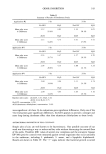
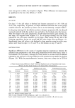
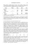
ANTIPERSPIRANT RESULTS 171 PCTREDofTversusC -- 100- (C - T)/C = 100- (1 - T/C) where T = sweat rate from the axilla treated with "test" product T, and C = sweat rate from the axilla treated with "control" product C. There are various statistical methods of treating the data to arrive at the mean sweat reduction and its statistical significance. FDA guidelines for antiperspirant efficacy (1-3) state that a product must attain strong evidence of a median sweat reduction (versus placebo or untreated) exceeding 20% in the user population to qualify as an effective antiperspirant (Category I). The antithesis is stated in terms of a statistical hypothesis as follows: Null hypothesis: Median sweat reduction is equal to or less than 20%. Rejection of this null hypothesis allows the experimenter to assert that the alternative hypothesis is true at a given confidence level, i.e., that the median sweat reduction is greater than 20%. The null hypothesis is tested at the significance level of 0.05 (one-sided). In competitive claims for advertising, the null hypothesis is that the sweat reduction of the candidate versus the competitor is equal to zero. If the hypothesis is rejected, then one of two alternative hypotheses are accepted: (a) that the sweat reduction exceeds zero, i.e., that the candidate has superior efficacy to the competitor, or (b) that the sweat reduction falls short of zero, i.e., that the competitor has superior efficacy. In this application, the null hypothesis is usually tested at the 0.05 significance level, two- sided. An early statistical method suggested by the FDA was the binomial test (1), but this method has fallen out of favor due to its low statistical power. Later, two other non- parametric tests were recommended by the FDA (3), based on the ranks of the ratios of sweat measurements of the right axilla to those of the left axilla: (a) the Wilcoxon rank sum test (Mann-Whitney test) on the ratios when no pretreatment data are taken, and (b) the Wilcoxon signed rank test on adjusted ratios when pretreatment data are taken. Both tests have reasonable statistical power, but unfortunately, neither test allows for easy calculation of confidence interval estimates for average percent sweat reduction. Another early method described by Majors and Wild (4) used the axillary sweat response ratios of test (T) to control (C) for each subject for normal-theory statistical tests, e.g., the Student t-test. These methods are currently in use, although criticized by Wood- ing (5) and Wooding and Finklestein (6) on the grounds that the T/C ratios do not have a normal distribution required for the valid use of such tests. A problem with arithmetic treatment of ratios is that the average result depends upon which treatment is placed in the denominator of the ratio. For example, consider the following results: Subject Sweat amount (mg) Ratio Ratio number Product A Product B A/B B/A 1 200 400 0.5 2.0 2 400 200 2.0 0.5 Average ratio 1.25 1.25 Average percent reduction 25 25

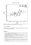
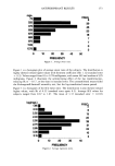
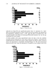
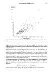
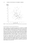
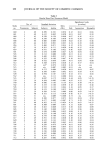
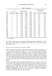
172 JOURNAL OF THE SOCIETY OF COSMETIC CHEMISTS If the ratio A/B is selected, then A appears inferior in efficacy to B but if the ratio B/A is selected, the reverse conclusion appears to be supported. In fact, from this limited data, most observers would conclude that the products were equivalent in efficacy. Post-treatment sweat response T/C ratios for each subject could also be adjusted by division by the corresponding pretreatment T/C ratios if the latter were available. Wooding and Finklestein (6) demonstrated that a logarithmic transformation of sweat rates resulted in normal distributions of the data and were valid for use in standard normal-theory hypothesis tests and confidence interval calculations. Wooding and Finklestein (6) were apparently the first writers to publish a mathematical model for the analysis of antiperspirancy data, which they called the "Sides Subjects Effects Model" (SSEM): Yjkm = •l• -3- 4)j -3- •k k -3- T m '-• Ejk m (our notation) where: Yjkrn is the logarithm of the sweat rate for axilla k of subject j, treated with treat- ment m, • is the log mean sweat rate over all subjects 4)j is the random effect of subject j, j = 1, . . . , n •k k is the fixed effect of sides (or laterality) k, k = 1,2 (left, right) q'm is the fixed effect of treatment m, m = 1,2 (control, test) {!jk m is the random effect of axilla k of subject j, treated with treatment m. subject to: ]E •kk= 0, • q'm = 0 k = 1,2 m = 1,2 4)i is N (0, tys=), independent, {jkm is N (0, ty=), independent, with qbj and •jkm mutually independent. NOTE: N (0, ty •) is statistical shorthand for the phrase: "Normally distributed with mean zero and variance ty 2." Wooding and Finklestein showed that this model removes the mean effects of sides and individual subjects from the error term. They recommended against the use of the simple baseline correction procedure. THE LOG TRANSFORM OF SWEAT MEASUREMENTS IS A NECESSITY The adoption of the logarithmic transformation of sweat rate was first proposed by Wooding (5) on the basis of his finding that the distribution of sweat rates was skewed, or asymmetrical, but became approximately symmetrical after log transformation. Fol- lowing computations in the log metric, the results could be back-transformed to the original metric. MacLennan and Whinney (10) have also confirmed the need for the log transform. Since Wooding's findings were based on relatively small data sets, we took our own 10ok at this question using close to 3000 baseline observations on 154 test subjects having ten or more baseline observations each. For each subject we calculated their average sweat rate and R/L ratios both in the original metric and the log metric.