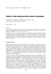
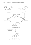
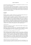
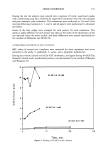
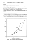
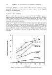
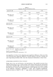
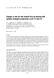
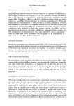
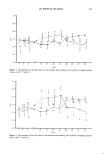
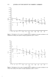
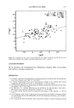
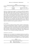
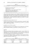
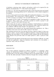
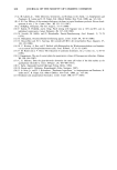
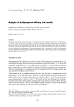
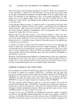
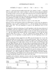
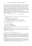
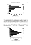
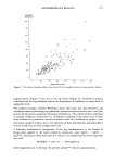
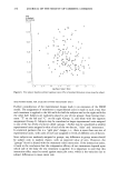
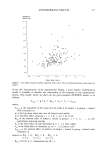
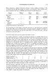
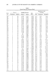
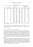
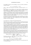
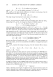
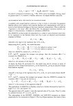
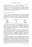
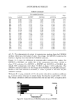
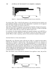
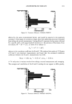
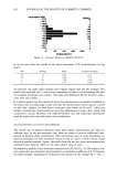
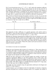
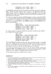
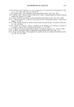
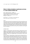
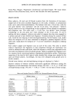
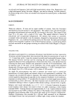
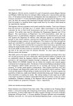
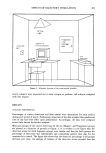
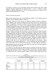
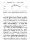
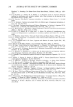
ANTIPERSPIRANT RESULTS 173 75 225 375 525 675 825 975 1125 1275 ! ......... ! ......... '! ......... i ......... i" ........ i lO 2o 3o 40 50 FREQUENCY Figure 1. Average sweat rates. 39 46 23 18 7 7 o 3 Figure 1 is a histogram plot of average sweat rates of the subjects. The distribution is highly skewed toward higher values with skewness coefficient (Sk) 1.12 (standard error = 0.2). Values ranged from 83 to 1278 milligrams, with mean 449 and median of 395 milligrams. Figure 2 illustrates the symmetrizing effect of the log transformation, reducing Sk to - 0.17, or less than its standard error. The untransformed means failed the Kolmogoroff-Smirnoff normality test, but the log-transformed means passed. Figure 3 is a histogram of the R/L sweat ratio. The distribution is also skewed toward higher values, with Sk of 0.52 (standard error again 0.2). Average R/L values for subjects ranged from 0.67 to 1.67. The mean of 1.13 (standard error = 0.013) 1.95 2.10 2.25 2.40 2.55 2.70 2.85 3.00 3.15 10 20 30 40 FREQUENCY Figure 2. Average log(sweat rates). FREQ. 2 6 13 25 39 31 22 10 3

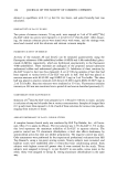
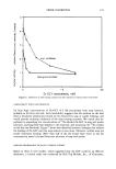
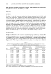
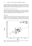
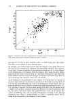
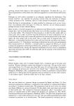
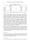
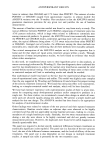
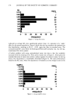
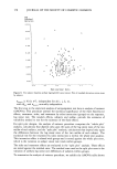
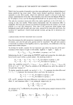
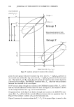
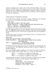
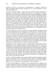
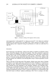
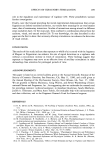
174 JOURNAL OF THE SOCIETY OF COSMETIC CHEMISTS 0.72 0.84 0.96 1.08 1.20 1.32 1.44 1.56 • 1.68 I ......... i ......... • ......... i ......... i ......... • ........ 0 10 • 30 40 ,50 GO FREQUENCY Figure 3. Average E/L ratios. FREQ. 1 7 18 8 3 2 indicated an average R/L ratio significantly greater than 1.0, indicative of a "sides" effect for the general population. Figure 4 shows that the log transform also symmetrizes this distribution, resulting in Sk of -0.09, again less than its standard error. The untransformed R/L ratios failed the Kolmogoroff-Smirnoff normality test, but the log- transformed R/L ratios passed. A further problem with using untransformed sweat rate data is that the variability increased with the sweating level. This can be clearly seen in Figure 5, which plots the standard deviation of sweat rates within a subject against the subject's mean. In the log metric this relationship is considerably diminished (Figure 6). The same phenomenon holds for the R/L ratio, where the dependence of variability on the average is seen in the -0.175 -0.125 -0.075 - 0.025 0.025 0.075 0.125 0.175 0.225 ......... ! ......... , ......... i ......... • ......... • ......... i 10 20 3o 40 50 6o FREQUENOY Figure 4. Average 1og(R/L ratios). FREQ. 1 1 4 51 4 2