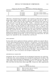
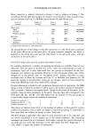
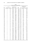
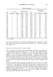
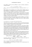
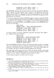
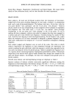
ANTIPERSPIRANT RESULTS 183 The confidence interval for the log difference in sweat rate between treatments is calculated as follows: Tp ñ t(l_ot/2,df) (Sp) [(1/n• + l/n2)] 1/' where t = upper 1-or/2 th percentile of the Student's t distribution with df = (n• q- n2 - 2). After calculation, the mean difference and its upper and lower confidence limits are back-transformed to the original sweat rate units of mg/20 min. Wooding and Fink- lestein (6) denoted this as Method A and presented a numerical example. A feature of the RRB design for multiple treatments is that estimates of Tp for each treatment pair come from two sources: (a) a direct estimate from the cell containing those two treatments, which is the same estimate as described above for the two- treatment case, and (b) an indirect estimate derived from pairs of cells having each treatment in common with another treatment. An example of an indirect estimate of treatments A and B is the difference in Tp between the AC cell and the BC cell. Indirect estimates have twice the variance of direct estimates and therefore require twice the sample size per cell to achieve precision equivalent to the direct comparison. USE OF BASELINE DATA--THE SIMPLE CHANGE FROM BASELINE MODEL When baseline data are available, it is desirable to make use of the information that they contain to increase the precision of the post-treatment analysis and to correct for possible bias due to imbalance in baseline R/L ratios between groups. It is true that random assignment of subjects to groups will, in the long run, balance differences in baseline R/L ratios among test groups. For any particular study, however, numerical differences in average baseline R/L ratio will always exist between groups due to measurement variation and random assignment, and the extent of these differences will vary for pairs of treatments. Since clients are only concerned with their study, not the long run, they are typically interested in checking for baseline differences and in making corrections where these differences occur. Earlier practitioners have been concerned about this and have suggested corrections for baseline effects. The form of baseline correction cited by Majors and Wild (4) was to divide the subject's right/left axillar post-treatment sweat ratio (Rp/Lp) by the corre- sponding right/left axillar baseline sweat ratio (Rb/Lb), resulting in a ratio of ratios. In the log metric this becomes a subtraction process, which is derived as follows: 1og{(Rp/Lp)/(Rb/Lb) } = log(Rp/Lp) - 1og(Rb/L b) = {1og(1 v) - log(L)}- {1og(10 - log(L0}. To develop a model for this simple change from baseline adjustment, first equate the baseline response, 1og(R b) - log(Lb), as: Bij = Yii• - Yii•' for subject j in group i, (Since no treatment has been applied the subscript m vanishes.) Using the POSTRT full model without the treatment term, and substituting for the Y's, the model becomes:

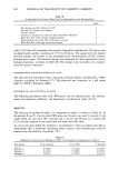
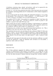
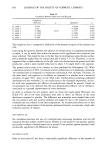
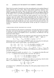
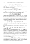
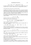
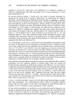
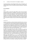
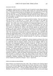
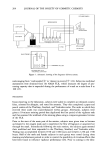
184 JOURNAL OF THE SOCIETY OF COSMETIC CHEMISTS Bii = k + ebii, for subjects in both groups, where k = 0% - k•), and the baseline variation •bij is N (0, trb2). If B•. and B2. are the mean baseline differences over subjects in each group, then the average baseline sides effect is estimated as: B.. = (B•. + B2. ) / 2. The simple change from baseline for each subject is the difference Cij = Pij - Bij, where Pij has previously been defined as the post-treatment sweat ratio log (Rp/Lp). Substituting for Pij and Bii , the change from baseline (CHGBAS) model is: Cli = 'r +½cti for subjects in group 1, and C2i = -'r + ½c2i for subjects in group 2, where the change from baseline variation ½•ii is N (0, ty•2), and 'r = (•2 - 'r l) is the previously defined treatment effect. There is no k term in the model, since we assume that the k terms for Pii and Bii are the same, namely the sides effect for the panel. The assumption that the k terms cancel could be questioned on the grounds that a treatment application could change the average sides effect for the panel. In this case we could represent the baseline sides effect as )kp and the post-treatment sides effect as )k b. The model would then become: Clj : ()kp -- )kb) •- 'I' -{- eclj for subjects in group 1, and C2j -- ()kp - )kb) -- 'r -t- e•2j for subjects in group 2. We have seen that the estimated value of )kp - )k b iS close to zero when averaged over the 70 past studies, and we have concluded that this difference is negligible and may be disregarded. -- -- If C•. and C2. represent the averages over groups, then the treatment effect is estimat- ed as: T• = (C•. - C2.)/2 = (P•. - P2.)/2 - (B•. -- B2.)/2 = Tp - T b -- __ where T b = (B1. - B2.)/2. Statistical calculations are then carried out as they were before for the POSTRT treat- ment effect, Tp. In the statistical literature this method is called the analysis of change (from baseline) and is discussed by Fleiss (9). Both the POSTRT (Tp) and CHGBAS (To) estimates are unbiased, i.e., both of their expected values are equal to 'r, and their difference has an expected value of zero. For any particular study, the POSTRT and CHGBAS estimates will be numerically different, since the baseline correction (Tb) is a random quantity that varies about its expected value of zero. It might be thought that the CHGBAS model will result in greater precision since it takes baseline variation into account, but this will not necessarily be so. The standard deviation of the CHGBAS model, ty• is' sqrt ((Tp 2 -t- (Tb 2 -- 2OpbO'pO'b) which is dependent on the degree of correlation of pre- and post-treatment values over subjects, measured by the correlation coefficient, Ppb- Therefore, the ratio of the baseline corrected standard deviation to the post-treatment standard deviation is: