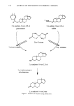
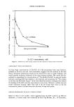
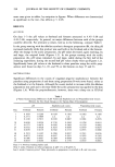
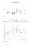
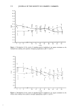
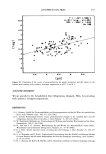
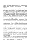
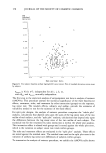
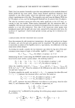
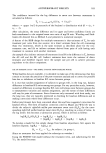
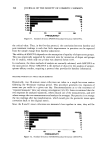
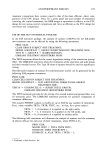
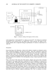
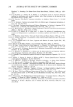
ANTIPERSPIRANT RESULTS 185 Crc/Cr p = sqrt (1 + 0 2 - 2ppt,0), where 0 = orb/or p. To achieve a reduction in variation, Ppb 0/2. If 0 is unity, for example, then Ppb must be greater than 0.5 to achieve a variance reduction via simple baseline correction. USE OF BASELINE DATA--THE ANALYSIS OF COVARIANCE MODEL A problem with simple baseline correction is that it tends to overcorrect for apparent baseline effects since subjects with extreme baseline ratio measurements will tend to revert to their historical average on their post-treatment measurement. This is called the "regression to the mean" effect [see Fleiss (9)]. An alternative statistical method, not subject to overcorrection, is analysis of covariance (ANCOVA). The ANCOVA method makes the adjustments to a subject's post-treatment sweat ratio Pij by regression on the baseline sweat ratio Bij to give an adjusted post-treatment response as follows: Paij = Pij -- •Bij, where •3 is the slope of the regression line of Pii on Bii. Substituting for Pii and Bij , the model becomes: Pa• i = M1 - •3) + 'r + ½a•i for subjects in group 1 and W2i = k(1 - •) - ß + e•2i for subjects in group 2, where the ANCOVA variation e% is N (0, If W and W represent the averages over groups, then the treatment effect ß is estimated by ANCOVA as: T• = (W•. - P•2.)/2 = {(P•. - P2.) - b(B•. - B2.)}/2 = Tp - bT• where b is the estimate of the slope As shown by Fleiss (9) and Laird (11), the model may also be written in terms of regression of the change from baseline Cii on the baseline B•i, giving an adjusted change from baseline response: caij = Ci j _ •t Bij, where •' is the slope of the regression line of Cii on B•i. It can be easily shown that =•-•. If C • and C•2 represent the averages over groups, then the ANCOVA estimate for ]. . treatment effect ß may also be written as: T• = (C•. - C•2.)/2 = {(C•. - C2.) - b'(B•. - B2.)}/2 = T c - b'T•, where b' is the estimate of the regression slope [3'. The applicability of ANCOVA to baseline correction is further discussed by Laird (11), Egger et al. (12), and Stanek (13). The expected value of T• equals 'r, since the expected value of Tb is zero. Thus T• is also an unbiased estimate of 'r, as is Tp and T c. The relationships of the POSTRT, CHGBAS, and ANCOVA estimates are shown graphically for two treatments in Figure 9. The two ellipses represent the cluster of data

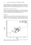
186 JOURNAL OF THE SOCIETY OF COSMETIC CHEMISTS PostTreatment LOG ( R 'C1. -a .•••Slope = 1 /..--$'"1"6"p e = b Group 1 Ellipses denote clusters of d•ta points for each of the tt•o õroup$ Group 2 51ope=l ...2 Baseline LOG ( R b / Lb) Figure 9. Graphical portrayal of treatment effect estimates. points for each group with post-treatment log sweat ratio Pii = 1og(Rp/Lp) plotted on the vertical axis and baseline log sweat ratio Bij = 1og(Rb/L b) plotted on the horizontal axis. The mean Pij and Bij values for each group are located at the center of gravity (centroid) of each ellipse. The POSTRT treatment effect, Tp, is half the vertical distance between the centroids of the two ellipses. If45 ø lines are drawn through each centroid, the CHGBAS treatment effect, T c, will be half the vertical difference between these two lines. In Figure 9, the estimate is shown at the average baseline ratio, L•, on the horizontal axis. If regression lines with slope b are drawn through each centroid, the ANCOVA treat- ment effect, T a, will be half the vertical difference between the two regression lines. In Figure 9 the estimate is shown at L• on the horizontal axis. Figure 9 portrays the situation where the Tc Tp. If the upper ellipse is moved to the