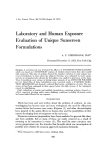
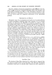
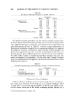
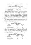
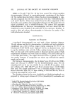
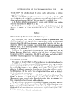
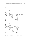
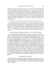
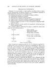
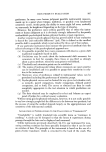
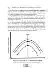
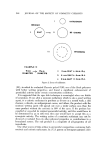
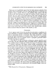
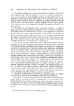
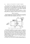
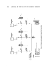
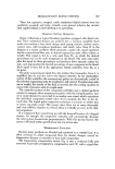
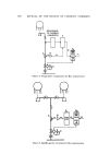
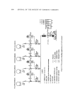
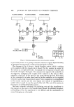
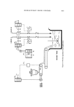
HIGH-ACCURACY BLEND CONTROL 597 These less expensive, compact, easily maintained digital systems were im- mediately accepted, and today virtually every process industry has success- fully applied digital in-line blending to its operations. BLENDING SYSTEM OPERATION Figure 3 illustrates a typical blending operation equipped with digital con- troI. Three individual streams are metered into a common manifold. Each meter run contains a base stock storage tank, pump, strainer, turbine meter, control valve with transducer/positioner, and check valve. Item D in the diagram is a master oscillator which generates a pulse rate signal represent- ing the required total flow rate, in desired engineering units, either volume or weight. This signal is fed to a ratio unit, Item D•, on which the desired percentages are set for each component in the blend. The ratio unit multi- plies the signal by these percentages and produces three separate output sig- nals, each representing the desired percentage of one component in the blend. Each signal is then fed to the appropriate digital controller, Item De as a set point. The pulse measurement signal from the turbine flow transmitter, Item A, is amplified, Item B, and also sent to the digital controller. In the standardizer section of the controller, the measurement pulses are electronically scaled to the selected engineering units for totalization and control. If engineering units are in weight, the density of the fluid is inserted into the scaling equation to convert the volumetric units to weight units. The controller portion of the component controller uses a digital up-down counter to compare these measurement pulses with the set-point pulses. Any error count detected is converted to an analog error signal which repositions the individual component control valve (C) to maintain the flow in the de- sired ratio. The digital pulse comparison technique is accurate to within pins or minus one pulse count. This means, since there are so many thousands, and even millions, of pulses in a blend, there is virtually no error in the digi- tal comparison. If a component flow cannot keep up with the demand because of a clogged strainer, for example, the component controller will automatically decrease the total system demand rate proportionately. With this pacing feature, the system will blend within specifications but at a slower rate. Measurement Correction Because many products are blended and marketed on a weight basis, it is often necessary to adiust component flows for density changes caused by temperature changes or variations in base stock composition. The temperature compensation circuit, Fig. 4, uses a resistance bulb and converter to provide a temperature compensation unit (E) with a signal that

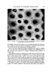
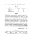
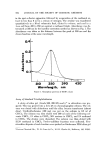
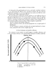
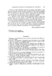
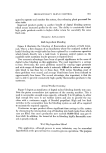
598 JOURNAL OF THE SOCIETY OF COSMETIC CHEMISTS ••__• R ESISTANCE TO-CURRENT A •. ,. •_.•_ I Figure 4. Temperature compensation for flow measurement L Figure 5. Specific gravity correction for flow measurement