282 JOURNAL OF THE SOCIETY OF COSMETIC CHEMISTS or in a more general form: where g(•) = kt (7) g(c) = f f(c) (8) As outlined earlier, a number of kinetic models have been derived that have subse- quently been found to apply to many solid-state reactions. A summary of the most common expressions is shown in Table I, with both the integral and differential form of the various equations being given. It is not intended to give lengthy proofs or descriptions of the various models in this publication however, should they be required, an excellent summary (with a full set of references) is given in reference 7. It can be seen that the models in Table I are grouped into three main categories: acceleratory, decel- eratory, and sigmoidal. These classifications are the first step in differentiating between the applicability of various expressions at the experimental level. An acceleratory reac- tion is one in which the maximum rate of reaction is in the later stages therefore, the rate is increasing over the majority of the reaction. Similarly, a deceleratory reaction is one in which the maximum rate is in the early stages of the reaction, meaning that the rate is decreasing over the majority of the reaction. Finally, a sigmoidal reaction is one in which the maximum rate is near the middle of the reaction. (It should be pointed out Table I Broad Classification of Solid-State Expressions Acceleratory or-time curves g(ot) = kt f(ot) = 1/k(dot/dt) P 1 Power law O/. 1/n n(o0(n -- 1)/n E 1 Exponential law In ot ot Sigmoidal or-time curves A2 Avrami-Erofeev [-ln(1 - ot)] •/2 2(1 - ot)(-ln(1 - or)) •/2 A3 Avrami-Erofeev [-ln(1 - ot)] v3 3(1 - ot)(-ln(1 - or)) 2/3 A4 Avrami-Erofeev I-In(1 - or)] v4 4(1 - ot)(-ln(1 - or)) 3/4 B 1 Prout-Tompkins ln[ot/(1 - or)] or(1 - or) Deceleratory or-time curves Based on geometrical models R2 Contracting area 1 - (1 - o0 ¾2 2(1 - or) v2 R3 Contracting volume 1 - (1 - or) •/3 3(1 - o0 2/3 Based on diffusion mechanisms D 1 One-dimensional ot 2 1/2or D2 Two-dimensional (1 - ot)ln(1 - or) + ot (-ln(1 - ot))-• D3 Three-dimensional [1 - (1 - ot)•/3] 2 3/2(1 -- 0/.) 2/3 (1 -- (1 -- O/.)1/3) --1 D4 Ginstling-Brounshtein (1 - 2ot/3) - (1 - o0 2/3 3/2((1 - or) -•/3 - 1) -• Based on "order" of reaction F ! First order - In(1 - or) 1 - ot F2 Second order 1/(1 - or) (1 - or) 2 F3 Third order [1/(1 - ot)] • 0.5(1 - o0 3

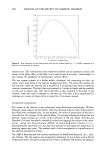
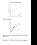
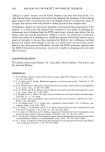
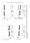
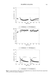
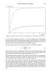
KINETICS OF HAIR REDUCTION 283 that the sigmoidal, acceleratory, or deceleratory nature of the reaction mechanism is not an indication of reaction-controlled or diffusion-controlled behavior.) The most popular method of identifying the appropriate kinetic model for a reaction is the reduced time method of Sharp et al. (8). Consider the integral form of the first order equation -In(1 - or) = kt (6) When ot = 0.5, this expression reduces to: 0.693 = kto. 5 (9) Using this expression as the normalizing function, i.e., dividing (6) by (9), then -In(1 - or) kt 0.693 - kt0.5 (10) or -In(1 - o0 = 0.693 t (11) t0.5 Hence master curves of or versus the reduced time (t/to.5) can now be constructed for the various theoretical mathematical models, and comparison of these master plots with the experimental data allows the best-fitting mechanism to be selected. Tables of reduced time data for the more common kinetic models have been given by Jones et al. (9). A slight modification of this method has also been proposed by Jones and coworkers in which either O/.experimental is plotted against O[theoretical, or (t/to.5)experimental is plotted against (t/to.5)theoretica 1 for a given model. Therefore, this method of analysis has the advantage that it gives rise to a more preferred linear relationship when the correct theoretical model has been identified. In this work we have used the more traditional method of Sharp et al. Using the integral form of the basic kinetic equation, Wickett has represented the pseudo first order reaction in terms of the tensile properties as rF(t)l -,n[F--•J = kC0t (12) Comparison of this equation with equation (6) shows that F(r)/F(0) can be equated to (1 - o0, and if the initial concentration (C o) is incorporated into the specific reaction rate constant, then both equations are the same. Similarly, the moving boundary model i IF(r)] 2 Cor3/2 n[F•-6•] - 3 k•- (13) can be expressed as [' ] - • In(1 - or) 2/3 = kt (14) if it is assumed that the temperature can also be incorporated into the constant. Therefore, the normalization can now be carried out to produce the theoretical reduced- time curves for these two models, as shown in Figure 1. To gain a better understanding of the physical significance of these two expressions, Figure 2 shows the derivative of these two plots expressed as a function of the fraction of reaction.