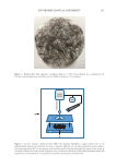
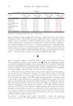
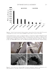
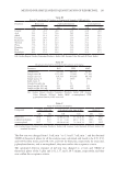
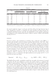
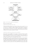
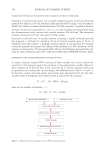
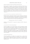
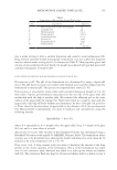
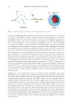
301 Characterizing and Modeling Complexion the “good complexion image” in each pair and then taking the logit function (log of odds, designated as Logit(A)) to transform the panel responses (in binary format) into a normally distributed dataset such that the probabilities of the panelists’ preferences were mapped to scales (ranging from negative infinity to positive infinity) and normally distributed (36,37). MODELING Statistical analysis and mathematical modeling were conducted using JMP-12, a commercially available statistical software package (SAS Institute, Cary, NC, USA). The standard least squares method was used to establish correlations between the panel-perceived differences, Logit(A), and the combined effects of skin visual attributes measured by image analysis. Since the panel results indicated the differences in image pairs, it was essential to match the properties of the measured skin attributes to those of panel responses. It was achieved by calculating the differences of the measured skin visual attributes for each image pair. Equation 1 shows the definition of such differences, where P represents any one of the objectively measured skin visual attributes A, B, or C represents the high-translucency-score group and X, Y, or Z represents the low-score group. Equation P P P e g., ITA° ITA° A B,orC X,Y,orZ A X 1. .,∆ =-∆ITA ° =-()The Bradley–Terry model, a probability model that can predict the outcome of a paired comparison (38–40), was employed to convert the Logit(A) results to a ranking order in terms of panel preference toward ideal complexion for the 36 study subjects. Image pairs of intra- and inter-group comparison necessary for the Bradley–Terry model but not covered in the original study design were created, and their corresponding panel preferences were simulated using the Logit model. JMP multiple linear regression was used again to correlate the preference ranks and the skin attributes to obtain a final model that can calculate ICS for each of the 36 study subjects. Figure 2 shows the flow chart of the modeling process. Table II Sample of Subject Pairing – Group 6 Pair ID Pair Translucency Score Age ITA° Value A, B, or C X, Y, or Z A, B, or C X, Y, or Z A, B, or C X, Y, or Z 61-La AX 5 7 56 56 21.6 22.5 62-L BX 4 7 54 56 29.8 22.5 63-L CX 5 7 54 56 27.7 22.5 64-L AY 5 6 56 47 21.6 24.4 65-L BY 4 6 54 47 29.8 24.4 66-L CY 5 6 54 47 27.7 24.4 67-L AZ 5 7 56 52 21.6 23.5 68-L BZ 4 7 56 52 29.8 23.5 69-L CZ 5 7 54 52 27.7 23.5 a Notation for pair ID: 6 =group number 1 =pair number L =high-score image placed on the left.

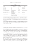
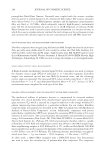
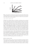
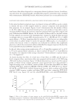
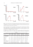
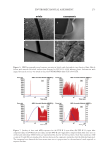
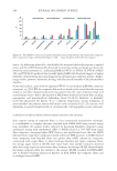
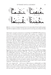
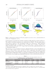
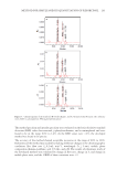
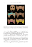
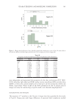
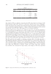
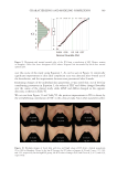
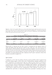
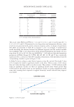
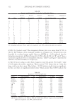
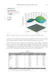
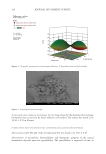
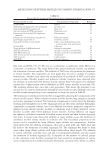
302 JOURNAL OF COSMETIC SCIENCE RESULTS AND DISCUSSION DISTRIBUTIONS OF SKIN TRANSLUCENCY SCORES Clinically graded skin translucency scores of the 36 subjects were in a range of 1 to 7 on a 10-point scale. Its distribution is shown in Figure 3A, which appeared to cover most of the scale and was considered acceptable for multiple regression analysis. The high–low pairs formed from the translucency scores showed a wide distribution of the differences between translucency scores in 54 paired images (Figure 3B), which provided various levels of difference in skin conditions for panelists to evaluate. DISTRIBUTIONS OF OBJECTIVELY MEASURED SKIN VISUAL ATTRIBUTES Image analysis on the facial ROIs of 36 study subjects resulted in raw datasets of various skin parameters. Shapiro–Wilk tests were performed as the first step of data analysis to check the normality of such datasets, and the key properties of their distributions are shown in Table III where values of the mean, standard deviation, W-value (a statistical parameter for normality test), and p value (probability) are listed. Since Shapiro–Wilk normality test assumed that a dataset was from a normal distribution (null hypothesis), a p value greater than 0.05 would not reject the null hypothesis. Therefore, the results in Table III indicate that all datasets were normally distributed, which was essential for numerical modeling. In addition, of the 11 attributes listed in Table I, three variables (L*, a*, and b*) were excluded from the modeling process due to their direct correlations with other variables such as ITA° and HUE. The remaining eight variables Figure 2. Flow chart of Ideal Complexion Score modeling process.