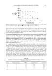
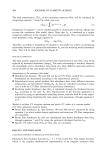
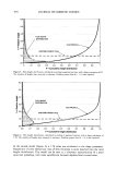
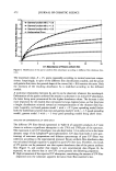
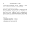
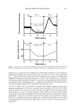
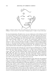
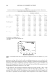
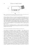
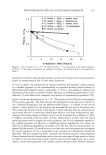
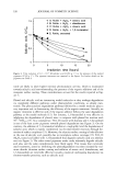
474 JOURNAL OF COSMETIC SCIENCE m 2,5 .o 2 .i • 1,{5 E .I e 1 ii • 0,{5 ß Sunscreen A ß Sunscreen B zx Sunscreen C ......................................................................................................... _ Gamma model with c = 1.5 x Sunscreenu , ß Sunscreen E I '•----------------•- © SunscreenF [ Gamma c = 1.5 ß ß ß ß ß ß ß ß ß i 0 2 4 6 8 10 12 14 16 18 20 A = Absorbance of Parent uniform film Figure 9. Experimental absorbance vs parent uniform film absorbance. Pairs of data were collected from sunscreens A-F, according to each studied wavelength. film) and spectroscopy in vitro (irregular film) can be assessed. AccoMing to the 23 sets of absorbance data, collected for each single sunscreen scan (290 to 400 nm, 5-nm increment steps), 138 pairs can be formed with the six sunscreen products. Figure 9 is a good example of experimental plot distribution, based on this type of UV graph. Both theoretical curves, based on gamma distribution with c = 0.5 and c = 1.5, are also reported on the same graph. We can note that all the individual data plots are well grouped and seem disposed around a single curve, whichever wavelength and sunscreen preparation is considered. Moreover, the shape of these experimental data plots is also remarkably similar to the shape of the mathematical curves previously studied. Therefore, the same kind of nonlinear relationship, already deduced from the theoretical models of sunscreen film distribution, can be experimentally assessed. As previously, the nonlinear relationship means that fragmentation of the uniform parent film results in a decrease in its potential UV absorbance, accoMing to absorption intensity. The decrease in the high UV absorption range is more intense than in the low UV absorption range. The 138 experimental data plots of sunscreens A-F are gathered just below the theo- retical gamma model curve with c = 1.5 (good spreading model). The result is obviously specific to the peculiar type of sunscreen vehicle used in our study (a normal O/W emulsion) and also depends on the in vitro spectroscopy requirements. We can also note that the efficiency of sunscreen vehicles can be assessed through the graph, mainly if the in vitro SPF is well correlated with the in vivo SPF. As an example, bad vehicles will achieve a lower set of experimental data plots, close to the model curve with c = 0.5. ADJUSTMENT OF THE CONTINUOUS FILM MODEL TO EXPERIMENTAL DATA The irregular film model, based on gamma height distribution, should be adjusted to achieve, for each data set, the smallest possible difference between experimental in vitro

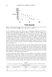
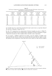
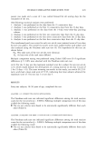
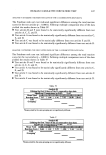
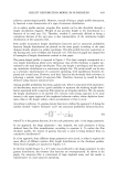
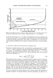
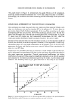
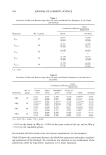
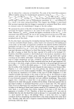
HEIGHT DISTRIBUTION MODEL IN SUNSCREENS 475 absorbance (Aexp)x and model absorbance (As)x, the latter being calculated according to parent film absorbance Ax. The shape parameter of the gamma function, from which the film geometry can be deduced, was adjusted through the 138 experimental sets of data of sunscreen preparations A-F. The final fit to the experimental data was determined by least-squares error assessment (equation 11): n=138 1 Amodel-- 1•8 x Z [(A:xp)X- (A•)X] 2 = minimum (11) An example of data treatment through Excel spreadsheet is given in Table II, with the 23 sets of UV data for sunscreen A. Every model absorbance data (As)x is calculated through numerical integration of equation 7 in which hv ) = inverse of gamma function, from F = 0 to F = 1. Total square error Arnodel , which is the sum of individual square errors (Aexpx-Asx) 2, should at least be reduced. This is accomplished by adjusting the shape parameter "c" via Excel Solver © (spreadsheet optimizer). As a matter of fact, all the 138 examples of suitable sunscreen data, from samples A to F, were finally added to the spreadsheet. According to this method, the film height distribution was successfully optimized, achieving a good correlation coefficient of 0.9960 with the experimental UV data, for a shape parameter of 1.105 (Figure 10). Table II Example of Spreadsheet Presentation with Absorbance Data of Sunscreen A Absorbance data Ax (Aexp)x (As)x hmode 1 Wavelength Parent film Experimental Calculated Square error 290 8.0100 1.4025 1.3869 0.0002 295 8.1437 1.4325 1.3944 0.0015 300 8.1388 1.3975 1.3942 0.0000 305 8.3059 1.3885 1.4034 0.0002 310 8.5248 1.4070 1.4153 0.0001 315 8.1676 1.3660 1.3958 0.0009 320 7.2331 1.3217 1.3407 0.0004 325 5.8371 1.2411 1.2446 0.0000 330 4.3124 1.1053 1.1115 0.0000 335 2.9423 0.9339 0.9487 0.0002 340 1.9024 0.7719 0.7731 0.0000 345 1.2263 0.6367 0.6114 0.0006 350 0.8006 0.5195 0.4726 0.0022 355 0.5245 0.4123 0.3554 0.0032 360 0.3326 0.3114 0.2534 0.0034 365 0.2042 0.2125 0.1708 0.0017 370 0.1188 0.1505 0.1067 0.0019 375 0.0682 0.0947 0.0643 0.0009 380 0.0380 0.0560 0.0371 0.0004 385 0.0211 0.0345 0.0211 0.0002 390 0.0115 0.0271 0.0118 0.0002 395 0.0067 0.0111 0.0071 0.0000 400 0.0036 0.0036 0.0040 0.0000 Total square error: 0.0183. Shape parameter: 1.105.