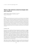
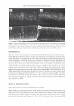
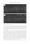
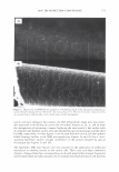
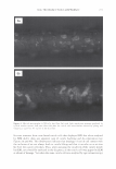
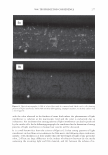
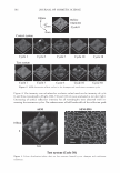
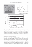
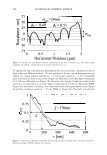
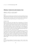
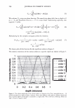
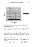
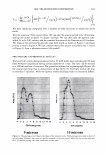
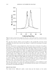
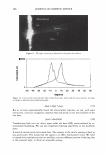
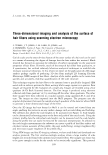
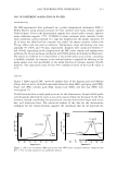
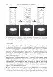
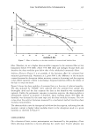
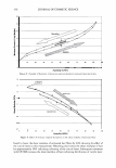
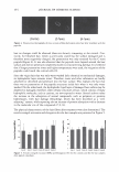
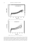
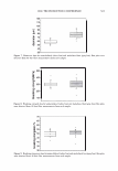
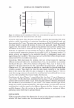
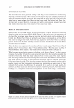
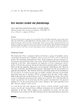
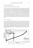
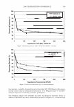
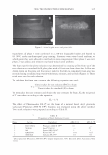
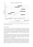
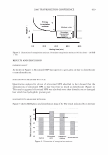
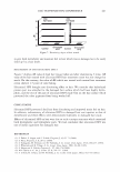
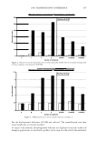
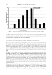
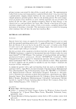
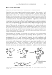
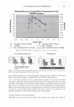
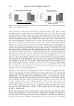
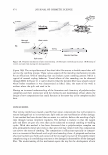
304 JOURNAL OF COSMETIC SCIENCE 0.30 0.25 7n 0.20 ::, 0.15 0.10 ..5 0.05 0.00 0 20 40 60 80 100 Scattering Angle (Deg.) Figure 9. Light scattering from a human hair. One trace is taken when the hair is oriented root-to-tip, while in the other the hair is reversed. Note both the ofhets in the peaks, and the structure that exists within them. The ring has structure which can be ascribed to the grating-like structure of the assemblage of cuticles that cover the hair. Figure 11 shows this scattering in the plane of incidence. We have observed the scattered light from a black Asian hair in the plane of incidence first using a 2.3-mm round hole and then after stepping the aperture down to a 0.5-mm slit. The aperture was about 40-mm away from the sample. These two traces are shown in Figures 12 and 13, respectively. Figure 13 is particularly interesting because it shows that we have enough resolution to extract the diffraction data directly. We do not have to depend upon the inferences that are found in data taken with coarse apertures. The relative heights of the "diffraction" peaks tell us how thick the cuticles are. This is an indication of hair wear assuming that the cuticles thin with abrasion or chemical attack. The width of the diffraction peaks (diffraction orders) gives us a measure of the variance in cuticle exposure. This is indicative of cuticle breakage, and thus a measure of hair damage as well. The broad background is associated with the creation of small defects, such as pitting, and has long been associated with loss of luster. We have thus shown that various hair damage mechanisms can be observed in and extracted from the light scattering data. The problem that now needs to be addressed is the removal of instrumental artifacts. DECONVOLUTION The width of the "diffraction" peaks 1s more than just the variance rn the cuticle

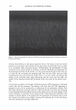
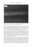
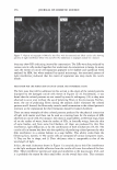
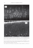
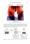
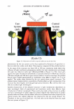
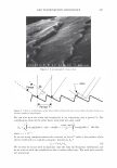
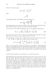
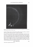
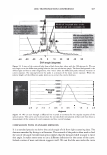
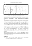
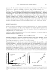
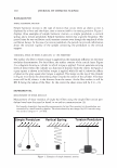
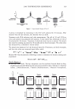
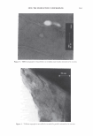
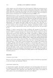
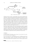
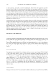
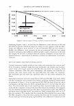
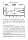
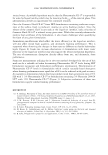
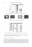
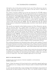
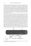
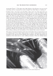
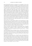
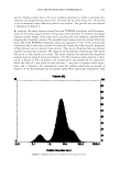
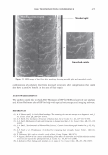
2006 TRI/PRINCETON CONFERENCE 305 Figure 10. Conical light scattering from a human hair. The hair's axis is perpendicular to the plane of the circle. The hair's axis pieces the circle's center. exposure. We have shown that the laser beam profile and aperture width are convoluted with the data. We will now show how to remove these effects. Our exposition has indicated that the convolution should appear in the form of error functions. It may be easier to simply measure the response function of the instrument. To do this, we simply need to pass our aperture across the laser beam. We can achieve this in our system by using a wire as our sample. We can thus scan across the diffracted line or circle that arises from the wire. Such a trace, along with a picture of the light pattern is shown in Figure 14. The trace is the impulse response of the optical system, which we can call H(0). We can take its Fourier transform, and label it h(w). The underlying data, or signal, can be denoted as G(0) while the raw data, D(0) is assumed to be the convolution of the two. We thus can write D(0) = H(0) Q9 G(0). (16) The Fourier transform then results in: