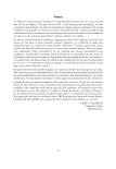
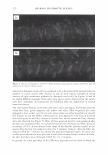
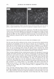
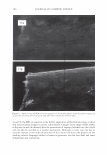
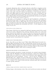
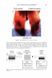
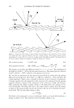
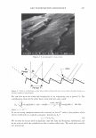
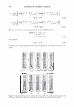
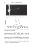
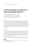
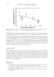
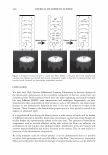
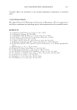
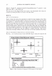
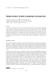
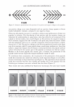
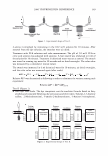
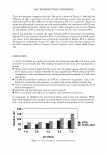
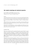
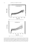
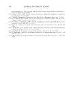
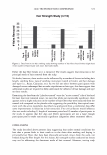
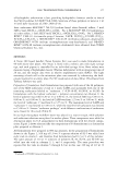
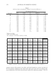
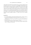
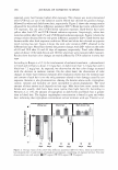
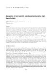
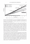
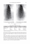
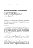
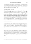
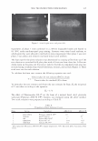
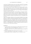
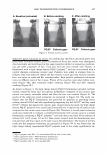
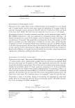
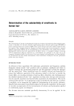
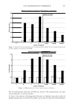
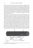
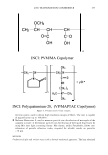
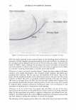
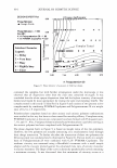
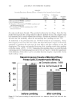
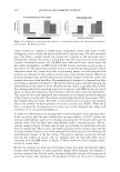
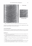
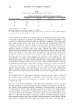
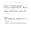
2006 TRI/PRINCETON CONFERENCE Given two Gaussian distributions, p 1 (x ) =- 2 1 exp[- (x - µ ) 2 ], 1TCJ 1 2CJ 1 pi (x ) = __exp[- 2 (x - µ ) 2 ]' 1TCJ 2 2CJ 2 their convolution is another Gaussian of broader variance and 301 (11) In our case the mean of the process is zero. The randomness of the grating that is the hair is noticed as an excess spreading of the laser beam. CONVOLVING THE BROADENED DIFFRACTED ORDERS WITH THE DETECTOR APERTURE Measurement systems have finite apertures. We can assume that this aperture is a slit of angular width 20, centered about and angle, a. For any given order, the detector sees a portion of the curve under the Gaussian intensity distribution as shown in Figure 6. This leads to a sum of error functions (ERF). a-8 a+8 a-8 a µ a µ I I I\ ) \ µ a+8 a+8 µa-8 Figure 6. The integral under the Gaussian can come in as a sum or difference of error functions depending upon the position of the aperture center relative to the location of the mean, and the aperture width.

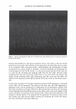
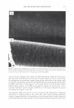
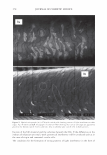
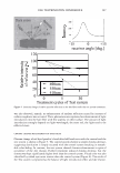
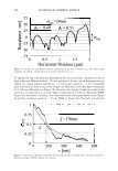
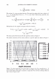
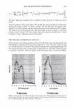
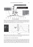
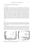
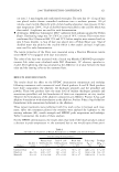
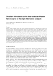
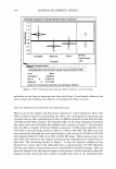
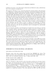
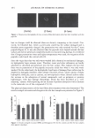
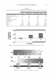
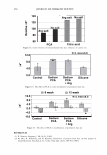
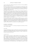
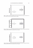
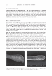
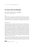
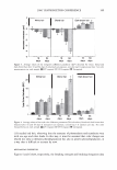
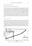
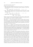
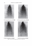
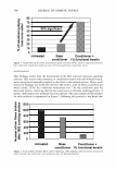
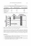
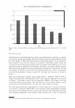
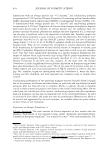
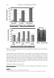
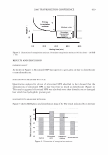
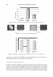
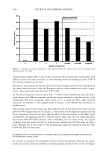
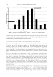
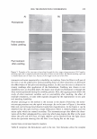
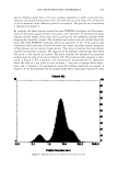
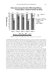
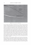
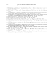
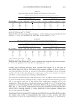
302 JOURNAL OF COSMETIC SCIENCE I = cr 0 { ERF('µ -al+&/ crv'z )-ERF('µ -aH/ crv'z)} for µ - al8 I = cr 0 { ERF(&-lµ -a'/ cry'z) +ERF('µ -al+&/ crv'z)} for +8 lµ-al We can write this in a more compact form using the SGN function. Let us define SGN(x) = -1 for x 0 = 0 for X = 0 = +1 for X 0 (12a) (126) (13) (14) Summing over all the significant orders (to /), weighted by their relative intensities, we obtain 0 0.1 .2 0.5 0.6 0.7 0.3 0.8 0.4 ·• O • I 12 SNII(_.. .. 0.85 Figure 7. Intensity plotted as a function of angle for various depths. The grating period was taken to be 10 microns. The indicated depths are in microns. The areas under the curves are nearly constant.